Talk:Mod:adb127
Introduction
Computational Chemistry allows us to perform calculations on systems that are too complicated to analyse by hand. In this exercise we will be using molecular dynamic simulation as our method for studying a simulation of a chemical system. This is a powerful method that will allow us to calculate thermodynamic properties for the system using a series of approximations which arise from the concepts of statistical physics. During molecular dynamics simulations we look at the way atoms move during a defined time period, using the positions, velocities and forces of the atoms to calculate the thermodynamic properties of interest.
Classical Particle Approximation
Approximations on the Schrödinger equation allow us to simulate a real system, usually to a relatively high level of accuracy when compared to experimental values. We must use approximations as exact solutions are simply not calculable for anything more complex than a hydrogen atom. The primary approximation we will use for this simulation is that atoms behave as classical particles. We assume that the atoms in the liquid act as a collection of N classical particles and as such apply Newton’s second law to them:
This equation then allows us to calculate the positions and velocities of the atoms in the system if we know how the force behaves as a function of time.
Numerical Integration
Because we have N atoms in our system, with N equations for each, we must approximate the quantity using discrete quantities to be able to solve the equations numerically. To do this, we break our simulation into a sequence of timesteps of length δt. To integrate Newton’s second law we use the Verlet algorithm which allows us to find the positions of the atoms to be found at timestep t+δt from a set of specified starting conditions. This method does not calculate the velocities of the atoms and as such prevents us being able to also calculate the kinetic energy of the system. To work around this we use a slight modification of the Verlet algorithm: the velocity-Verlet. This works on the assumption that the acceleration of an atom is dependent only on its position and not its velocity.
TASK: Open the file HO.xls. In it, the velocity-Verlet algorithm is used to model the behaviour of a classical harmonic oscillator. Complete the three columns "ANALYTICAL", "ERROR", and "ENERGY": "ANALYTICAL" should contain the value of the classical solution for the position at time, "ERROR" should contain the absolute difference between "ANALYTICAL" and the velocity-Verlet solution (i.e. ERROR should always be positive -- make sure you leave the half step rows blank!), and "ENERGY" should contain the total energy of the oscillator for the velocity-Verlet solution.
TASK: For the default timestep value, 0.1, estimate the positions of the maxima in the ERROR column as a function of time. Make a plot showing these values as a function of time, and fit an appropriate function to the data.
The three graphs below show the position as calculated using the classical harmonic oscillator, the Velocity-Verlet algorithm and the error between the two methods. The energy shown here is calculated as the sum of the potential energy and the kinetic energy at each point.
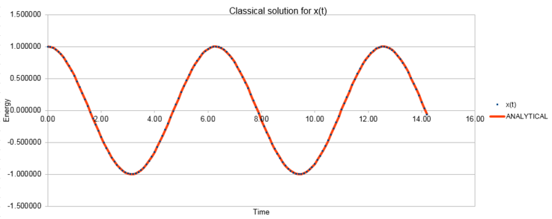
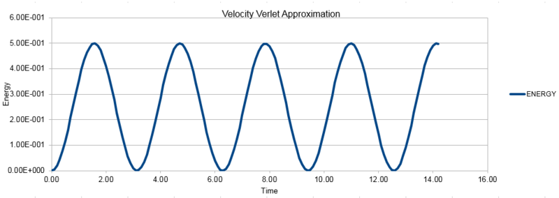
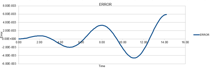
NJ: This was meant to the the absolute error so that you could make a fit to the maxima.
TASK: Experiment with different values of the timestep. What sort of a timestep do you need to use to ensure that the total energy does not change by more than 1% over the course of your "simulation"?
Experimentation shows that the timestep must be kept under 0.2 in order to keep the total energy within 1% over the course of the simulation, as at a timestep of 0.2 the energy changes exactly 1% during the simulation.
Why do you think it is important to monitor the total energy of a physical system when modelling its behaviour numerically?
It is important to monitor the total energy of a physical system as we anticipate a conservation of energy from using Newton’s second law but instead of a simple conservation of energy, we actually see energy fluctuations both in the short term and long term. We must monitor this to ensure there is no significant energy drift leading to unreliable simulations. As such, we see that the Velocity-verlet algorithm actually has a good stability in the long term.
Atomic Forces
It is necessary to make approximations to study the forces acting on the atoms in our simulation. To study force in classical physics we use the equation:
The function that we use for U, the potential, comes from the Lennard-Jones potential which acts as a decent approximation for simple liquids.
TASK: For a single Lennard-Jones interaction, find the separation at which the potential energy is zero. What is the force at this separation? Find the equilibrium separation, and work out the well depth.
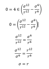
Thus factoring in to the force equation
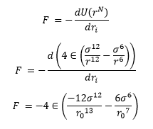
Using:
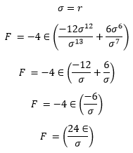
Equilibrium Separation (req) is the value at the minimum of the curve, and thus is the value when the first derivative (Force) equals zero
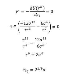
The well depth is then the value of ø at the equilibrium distance so we substitute the value of r_eq into the Lennard-Jones equation equation
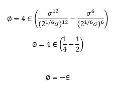
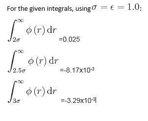
NJ: Show a bit more working.
Periodic Boundary Conditions
We are not able to run simulations on large numbers of atoms because of the computational demand. As such, we are not able to simulate real volumes of liquids, and instead will run simulations containing 1000 to 100000 atoms. To allow for the approximation of real volumes of liquid within the scope of our computational ability, we apply periodic boundary conditions. We treat our atoms as though they are enclosed in in a box of fixed dimensions repeated infinitely in all directions. When an atom crosses the boundary of the box it is replaced instantly by a replica on the opposite face thus ensuring the number of atoms remains constant within the box.
TASK: Estimate the number of water molecules in 1ml of water under standard conditions. Estimate the volume of water molecules under standard conditions.
1ml = 1g of water
Mr of H2O = 2+16 = 18 g/mol
Thus in 1ml of water, there are 1/18 moles of water
Using Avogadro’s number: 6.0221409x10²³
Number of molecules in 1g:
= 1/18 * 6.0221409x1023
= 3.35x10²² molecules
Calculating Volume of 1000 water molecules:
Number
of moles
= 10000/(6.0221409x1023)
= 1.660539x10⁻²⁰
Mass = Moles*18gmol-1
=1.660539 x10-20*18 g
= 2.9889703x10⁻¹⁹g
1g = 1ml = 1cm3
Thus volume = 2.99x10⁻¹⁹ cm3
TASK: Consider an atom at position in a cubic simulation box which runs from to. In a single timestep, it moves along the vector. At what point does it end up, after the periodic boundary conditions have been applied?'
The atom ends up at (0.2, 0.1, 0.7)
Truncation
We often use the approximation that there is a distance beyond which the interaction between atoms is so small that we can safely ignore it. In most simulations this distance is chosen to be something close to 3σ, after which distance we ignore the atoms present when performing our force calculations.
TASK: The Lennard-Jones parameters for argon are σ = 0.34nm, ε/kB = 120K. If the LJ cutoff is r* = 3.2 what is it in real units? What is the well depth in kJ mol-1? What is the reduced temperature T*=1.5 in real units?
Using distance reduction r* = r/σ , 3.2 = r/0.34nm , thus distance = 1.09nm
Well depth = -ɛ , -ɛ =120*kB*NA/1000 = 0.10Kj/mol
NJ: Careful with the capitals - it's kJ, not Kj.
Temperature T* = kBT/ɛ , 1.5= 1*T/120K , 180K = T
Equilibration
TASK: Why do you think giving atoms random starting coordinates causes problems in simulations? Hint: what happens if two atoms happen to be generated close together?
If we gave atoms completely random starting coordinates, there is a chance that atoms would end up too close together and thus their overlapping potentials would produce a very high energy. This may mean that instead of the system reaching an equilibrium the simulation would ‘explode’ as the energies are much higher than could actually exist in a real liquid. We thus run our simulations using atoms as though they are on the lattice points of the material in its solid state that we then melt to the liquid.
For example, as in the exercise where using the command lattice sc 0.8, we use a solid with simple cubic lattice with spacing number 0.8, we get the spacing between the lattice points in the output file as 1.07722 in reduced form.
TASK: Satisfy yourself that this lattice spacing corresponds to a number density of lattice points of . Consider instead a face-centred cubic lattice with a lattice point number density of 1.2. What is the side length of the cubic unit cell?
To work out the lattice density we must work out the volume of the cube relating to the lattice spacing and compare it to the unit cell. The value for spacing between lattice points for a cubic lattice can also be treated as the length of any side of the cube. Thus the volume of the cube must be 1.077223 = 1.25, using V=a3
Examples of the code used
Comparing this to the unit cell which we know contains one atom we can calculate the number density as 1/1.25 = 0.8
A face centred cubic lattice contains four atoms. By utilising the number density we find that the volume of the cube must be 4/1.2 = 3.33, so using V=a3 each side must have length 1.5 in reduced units.
NJ: To 2 s.f.
TASK: Consider again the face-centred cubic lattice from the previous task. How many atoms would be created by the create_atoms command if you had defined that lattice instead?
In the task, the simulation box is based around a simple cubic lattice which contains only one atom. The box contains 1000 unit cells and so contains 1000 atoms. The face-centred cubic lattic has four atoms in each unit cell, and so the create_atoms command must generate 4000 atoms .
TASK: Using the LAMMPS manual, find the purpose of the following commands in the input script:
mass 1 1.0
pair_style lj/cut 3.0
pair_coeff * * 1.0 1.0
mass 1 1.0
Sets the mass for the atom as 1.0. It is a command of general form where I specifies the atom type, as in this example an explicit numeric value is set, though a wild-card asterisk can be used to set the mass for multiple atom types.
pair_style lj/cut 3.0
pair_style sets the formulas LAMMPS uses to calculate interactions between atoms. The addition of lj/cut 3.0 means that this command refers to the interaction of the pair potentials between pairs of atoms using the Lennard-Jones potential with a cut off at 3 distance units.
pair_coeff * * 1.0 1.0
pair_coeff specifies the coefficients for the pairwise force field for one or more pairs of atom types. With the asterisk again acting as a wild card, this command sets the coefficients for all atom pairs in the simulation to 1.0.
NJ: What are the coefficients in this case?
TASK: Given that we are specifying xi(0) and vi(0), which integration algorithm are we going to use?
Because we are specifying both position and velocity starting values we cannot simply use the Verlet algorithm so must use the Velocity-Verlet integration algorithm.
TASK: Look at the lines below.
### SPECIFY TIMESTEP ###
variable timestep equal 0.001
variable n_steps equal floor(100/${timestep})
variable n_steps equal floor(100/0.001)
timestep ${timestep}
timestep 0.001

### RUN SIMULATION ###
 run ${n_steps}
 run 100000
The second line (starting "variable timestep...") tells LAMMPS that if it encounters the text ${timestep} on a subsequent line, it should replace it by the value given. In this case, the value ${timestep} is always replaced by 0.001. In light of this, what do you think the purpose of these lines is? Why not just write:
timestep 0.001
run 100000
By defining the timestep using the text ${timestep} we can control the value of the timestep throughout the input script. By fully defining the timestep at this point, it is then consistently defined for the whole simulation in which the timestep may be repeated with reference to a variety of other commands. It also allows us to simply and easily change the timestep to compare how this changes our output by altering a single command to run the whole simulation rather than in many separate commands.
NJ: This section makes sure that you always simulate the same time (nsteps*dt), no matter what timestep is chosen.
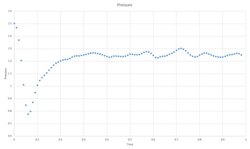
TASK: make plots of the energy, temperature, and pressure, against time for the 0.001 timestep experiment (attach a picture to your report). Does the simulation reach equilibrium? How long does this take?
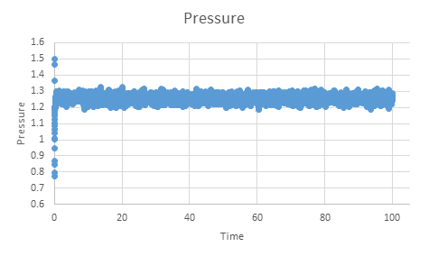
NJ: This graph might be slightly clearer with (thin) lines rather than points.
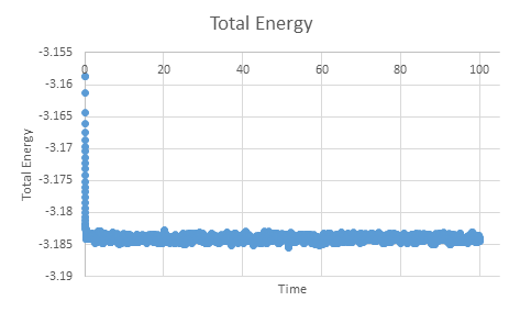
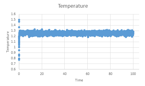
If we zoom in on the plot for pressure we can see that equilibrium is reached within the simulation within approximately 0.5 time units.
When you have done this, make a single plot which shows the energy versus time for all of the timesteps (again, attach a picture to your report).
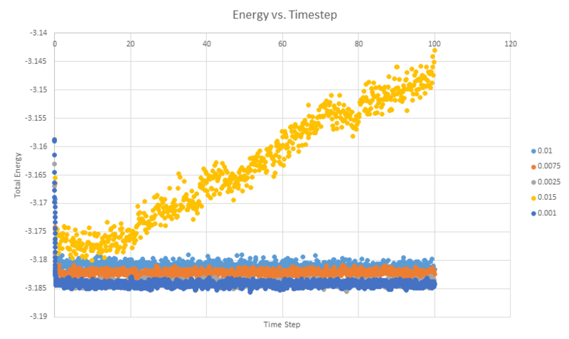
Choosing a timestep is a balancing act: the shorter the timestep, the more accurately the results of your simulation will reflect the physical reality; short timesteps, however, mean that the same number of simulation steps cover a shorter amount of actual time, and this is very unhelpful if the process you want to study requires observation over a long time. Of the five timesteps that you used, which is the largest to give acceptable results? Which one of the five is a particularly bad choice? Why?
The largest time step of the five that gives acceptable results is the 0.01 timestep. 0.015 is a particularly bad choice as it does not actually reach an equilibrium and instead continues increasing in energy. In the longer timesteps, the atoms are more likely to move into an energetically unfavourable in any given timestep. In too large a timestep, atoms may be forced to move to a point where their potentials overlap which causes a very large force, driving the atoms apart.
NJ: 0.01 is a bit big. We don't really want the average energy to depend on the choice of timestep - the two smallest timesteps, 0.001 and 0.0025 should give approximately the same results. 0.0025 is then the best choice because we get more time out of the simulation for the same number of steps.
Running simulations under specific conditions
We will now move on from the microcanonical system with which we have been working so far and look at how the system changes under particular experimental conditions. We will run simulations under the npT ensemble, which will allow us to sketch an equation of state for the simulation at atmospheric pressure.
To control the temperature of the system, the instantaneous temperature, T, must be calculated at the end of each timestep and used to calculate the value of γ. This constant will then be used to bring the temperature to the target temperature by multiplication.
TASK: We need to choose γ so that the temperature is correct T = if we multiply every velocity γ. We can write two equations:
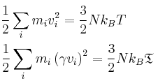
Solve these to determine γ.
The second equation can be divided by the first giving γ2 = T/
And therefore γ = (T/)1/2
NJ: Show a bit more working.
To calculate the equation of state, we need the temperature, density, pressure and standard errors for each to be specified. The lines used for this are as follows:
### MEASURE SYSTEM STATE ###
thermo_style custom step etotal temp press density
variable dens equal density
variable dens2 equal density*density
variable temp equal temp
variable temp2 equal temp*temp
variable press equal press
variable press2 equal press*press
fix aves all ave/time 100 1000 100000 v_dens v_temp v_press v_dens2 v_temp2 v_press2
run 100000
TASK: Use the manual page to find out the importance of the three numbers 100 1000 100000. How often will values of the temperature, etc., be sampled for the average? How many measurements contribute to the average? Looking to the following line, how much time will you simulate?
The three number 100, 1000, 100000 correspond to the general input commands Nevery, Nrepeat and Nfreq respectively. The use of 100 tells the programme to use input values every 100 timesteps, meaning the programme will take samples of temperature, pressure etc. every 100 timesteps. The use of 1000 indicates that the input values for calculating averages should be used 1000 times. 10000 is the timestep between calculations of averages. This command in its entirety thus instructs us to take a sample every 100 steps 1000 times until 100000 steps have passed. We will only get one average value output from this specific command as 100*1000=100000.
Plotting the Equations of State
TASK: When your simulations have finished, download the log files as before. At the end of the log file, LAMMPS will output the values and errors for the pressure, temperature, and density (N/V). Use software of your choice to plot the density as a function of temperature for both of the pressures that you simulated. Your graph(s) should include error bars in both the x and y directions. You should also include a line corresponding to the density predicted by the ideal gas law at that pressure. Is your simulated density lower or higher? Justify this. Does the discrepancy increase or decrease with pressure?
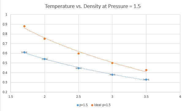
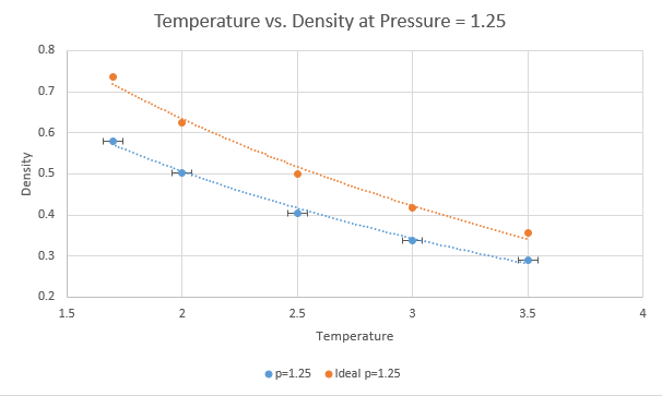
The plots above show five temperatures (1.7, 2.0, 2.5, 3.0, 3.5) and two pressures (1.25, 1.5) under the npT ensemble. Each plot has error bars in both directions from the output file but the vertical error is much too small to be shown on the scale used.
The simulated density is lower than that predicted by the ideal gas law at both pressures and all temperatures. This is because there will be interactions taking place between atoms that are not taken into account in the ideal gas law. The discrepancy between real and ideal increases with decreasing temperature. This is because at higher temperatures, atoms act as though there are fewer interactions because the molecules will have their interactions dominated by kinetic energy. There is negligible difference seen here between ideal and real with respect to pressure, though it can be assumed that at lower densities atoms will be further apart and so will interact less, and as such lower densities will have less discrepancy between the ideal and the observed.
NJ: Did you fit a function to the ideal gas law?
Heat Capacity Calculation

Heat capacity [1] is a property of a system that is related to the fluctuation from the average value and is described by the above equation. To be able to run a simulation that calculates heat capacity we must modify the input scripts we have used for previous simulations. We now need a simulation that runs under the NVT ensemble. To allow for this, density of the lattice is added to the list of variables controlled in the commands. The average energy and the energy squared are printed to the output to allow the heat capacity to be calculated.
An example input script can be found here:
[[1]]
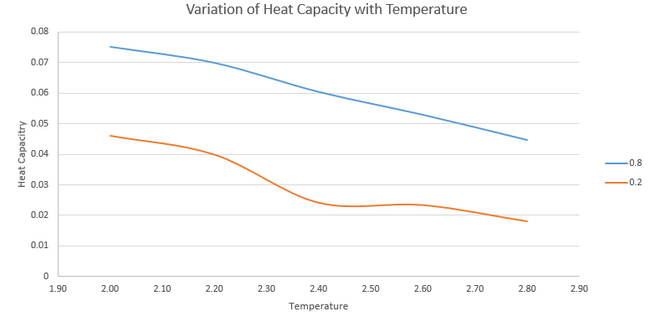
NJ: You shouldn't use the Excel "smooth lines" in plots like this - do you think the kink is really part of the trend, or the result of measurement error? You could fit a line or curve instead, if you wanted to.
The graph shows that higher density correlates to a higher heat capacity. This is to be expected because there are a higher number of atoms per unit volume at a higher density and heat capacity is an extensive property so is higher when more atoms are present.
NJ: What about the trend with temperature?
TASK: As in the last section, you need to run simulations at ten phase points. In this section, we will be in density-temperature phase space, rather than pressure-temperature phase space. The two densities required at 0.2 and 0.8, and the temperature range is 2.0, 2.2, 2.4, 2.6, 2.8. Plot CV as a function of temperature, where is the volume of the simulation cell, for both of your densities (on the same graph). Is the trend the one you would expect? Attach an example of one of your input scripts to your report.
Structural Properties and the Radial Distribution Function
In this simulation we explore the structure of our system using the radial distribution function. The radial distribution function describes the likelihood of finding an atom at a distance, r, from a reference point in an ideal gas. It can also be used as a way to describe the density of the system as a function of the distance from a reference point.
TASK: perform simulations of the Lennard-Jones system in the three phases. When each is complete, download the trajectory and calculate and. Plot the RDFs for the three systems on the same axes, and attach a copy to your report. Discuss qualitatively the differences between the three RDFs, and what this tells you about the structure of the system in each phase. In the solid case, illustrate which lattice sites the first three peaks correspond to. What is the lattice spacing? What is the coordination number for each of the first three peaks?
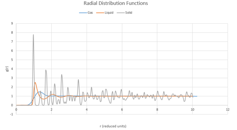
The program VMD is used to plot g(r) and its running integral Int(g(r)) using Lennard-Jones system simulations in the three phases (liquid, gas, solid). Each input script was given different densities and temperatures to produce the phases. Cubic lattice was used for gas and liquid phases, and face centred cubic was used for the solid phase.
The gas atoms do not have any long range regular spacing, though do have some particles close to each other as indicated by primarily a flat value with one peak.
The solid has a regular, ordered lattice structure and so the peaks fall at regular intervals with the first peak close to starting position. Each peak corresponds to the nearest neighbour in the solid and lines up with the structure of the solid's crystal form.
The liquid is an intermediate curve between the solid and gas, with clearly a few interactions with nearby atoms but not as many or as regularly structure as for a solid.
For all states, we can see that there is nearly no likelihood of finding a nearby atom for the shortest distances which can be explained by the fact that it is energetically unfavourable to have two atoms so close together.
NJ: We generally classify the phases as follows: gas, no order; liquid, short range but no long range order; solid, short and long range order.
Using the plots for the solid of RDF we can determine the coordination number of the nearest neighbours to the atom we are studying by looking at the points where the peaks collapse. In this case these peaks are at 1.05, 1.40, and 1.75. Cross-referencing these r values with the running integral and subtracting the areas of the relevant preceding peaks gives us coordinations of 12, 6 and 24.
NJ: It would be nice to see the plots showing these. NJ: What neighbours in the crystal do these peaks correspond to?
By study of the face-centred cubic, we see that the second nearest neighbour is on the lattice edge and as such, the distance corresponds to the lattice spacing. This gives us a lattice spacing value of 1.45.
NJ: Once you know which neighbours give rise to which peaks, you can work out the three distances in terms of a. You can then average over three different estimates of a.
Dynamical Properties and the Diffusion Coefficient
The diffusion coefficient of our simulation can be calculated using the mean square of displacement r2 which is a measure of the random movement of our atoms across the course of the simulation.
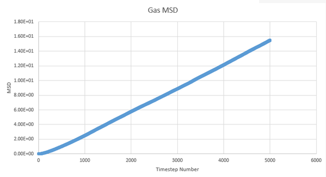

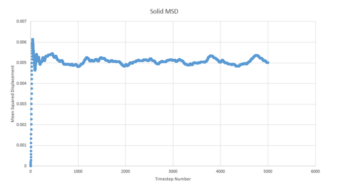
NJ: Why is the vapour curve slightly curved at the beginning?
NJ: Because you've plotted against timestep, not time, you have a diffusion coefficient in terms of distance squared per timestep.
These graphs of mean squared displacement plotted as a function of timestep allow us to estimate the diffusion coefficient. To do so, we measure the gradient at a point on the plot of approximate linearity and multiply it by 1/6. This gives approximate values of 50, 1.52x10⁻³ and 5.12x10⁻¹⁰ for gas, liquid and solid.
NJ: This is a very large discrepancy, what do you think its origin is?
This is as we would expect, as simple consideration of the freedom of motion for atoms in each state can explain the difference in displacement values. In a gas, the atoms are free to move and so the diffusion coefficient is much higher than for a solid where the atoms are restricted to vibration within their regular lattice structure with liquid providing an intermediate value as an intermediate state in which the atoms can move relatively freely but do not have complete freedom of motion.
Because mean squared displacement is a value that we expect to progress in a linear fashion due to the atom moving at a regular pace, we expect the graph of this to be linear. This is largely what we see though there is a small disruption at the start as the system reaches equilibrium.
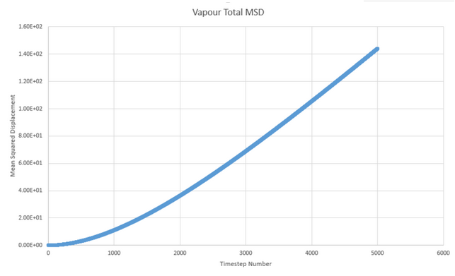
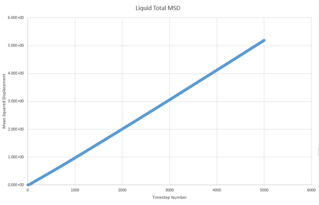

These graphs are for the million atom system. There is little difference between the simultaions other than the plots appearing more smooth for the plots with more atoms. Whilst the trend is maintained, the values of the diffusion coefficient are in fact relatively different with new D values of: 5.08x10⁻³ 1.83x10⁻⁴ and -1.68x10⁻⁸.
Velocity Auto Correlation Function
The velocity auto correlation function is another method by which to calculate the diffusion coefficient. We simply integrate the function:

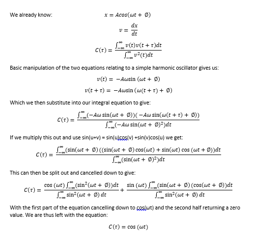
TASK: In the theoretical section at the beginning, the equation for the evolution of the position of a 1D harmonic oscillator as a function of time was given. Using this, evaluate the normalised velocity autocorrelation function for a 1D harmonic oscillator (it is analytic!):

Be sure to show your working in your writeup. On the same graph, with x range 0 to 500, plot C(tau) with ω = 1/2π and the VACFs from your liquid and solid simulations. What do the minima in the VACFs for the liquid and solid system represent? Discuss the origin of the differences between the liquid and solid VACFs. The harmonic oscillator VACF is very different to the Lennard Jones solid and liquid. Why is this? Attach a copy of your plot to your writeup.
If we take the value of ω to be 1/2π in the harmonic oscillator and plot using the above equation the VACF for a solid and a liquid alongside the harmonic oscillator we get the following graph:
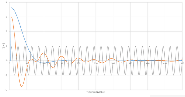
For the two plots from our equation, we can understand the shape of the curve by considering what is taking place during the simulation. The plots both start with a rapid drop which is due to the velocity of the atoms changing after collision. Relating to this, the liquid plot reaches a negative minimum that is not as present in the solid before reaching equilibrium. The minima on the plot reflect the collisions that take place with a large angle of deflection (approx 180o).
The differences between the solid and liquid plots primarily stem from the freedom of motion for the atoms in the system. In the liquid the atoms are relatively free to move and so the VCAF for a liquid decays to zero much faster. For the solid, the atoms are constrained by the lattice structure in which they sit.
The harmonic oscillator does not factor in any external forces so does not undergo collisions or self diffusion. It is thus a useful comparison tool as when the shape of the solid resembles the shape we know that it must be because the solid atoms are being less affected by external forces. This is to be expected as the only external forces able to be exerted on the atoms in the solid are to cause vibration within the structure and small intramolecular forces from neighbouring atoms.
NJ: Good NJ: The negative regions of the VACF correspond to collision with other atoms. The single minimum in the liquid VACF is due to collision with the "solvent cage".
NJ: There's nothing for the HO to collide with, so its velocity can never become decorrelated.
TASK: Use the trapezium rule to approximate the integral under the velocity autocorrelation function for the solid, liquid, and gas, and use these values to estimate D in each case. You should make a plot of the running integral in each case. Are they as you expect? Repeat this procedure for the VACF data that you were given from the one million atom simulations. What do you think is the largest source of error in your estimates of D from the VACF?
Gas plot: D ≈ 3.42
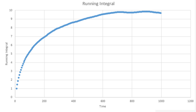
Liquid plot: D ≈ 8.10 x 10⁻¹
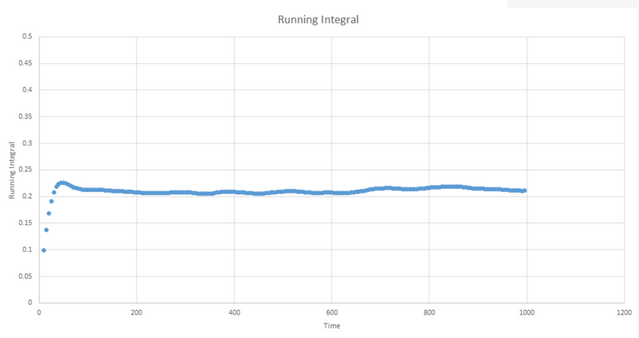
Solid plot: D ≈ 5.73 x 10⁻⁴
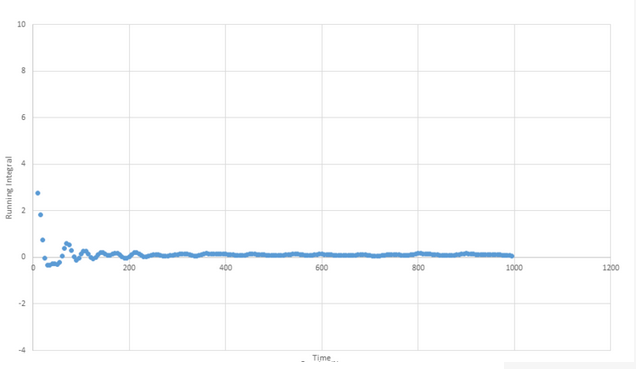
The most likely cause of error stems from the fact that the graphs all decay to a near zero value within a relatively short timescale but take a lot longer to actually reach zero. This will mean that for almost all time ranges at which we are likely to measure, we will likely underestimate D because we will perform an integration that does not capture all the data until the plot finally reaches zero. The MSD values will be less of an underestimate as they are gradient based rather than integration based.
NJ: Very well spotted!
[1] Atkins, Physical Chemistry, Ninth Edition, Oxford University Press
