Talk:Mod:ZG CMP Monte Carlo Sim
JC: General comments: This is a brilliant report, well done. You show that you have a very good understanding of the theory of the Ising model and that you understand each step of the experiment. You also manage to include a lot of extra material and analysis. ZG: At the bottom of the page there is a box containing the code that was used to estimate the the Curie temperature. Was this not sufficient? Could you give another example were I missed or failed to complete part of the tasks, I am failing to see them myself? JC: Please wait until I've finished marking, that comment was from a previous report, I just copied it onto yours to make sure the formatting for my comments is consistent. ZG: My apologies
Ising Model
Lowest Energy
A minimum in energy is reached when all spins are of the same sign. The sign of the spins should not matter, owing to the product of two negative spins being positive. Energy shall be negative for these states, provided is positive (taken to be 1 in this case), owing to the negative sign in equation 1 and positive summation of spin; where , , and are the energy, interaction constant, number of spins and spin, respectively.
(1)
Each atom in the 1D Ising lattice model has 2 neighbours, owing to the boundary conditions ensuring periodicity holds for the whole lattice. In 2D, each atom has 4 neighbours, and in 3D there are 6. Taking all of the spins as the same sign results in the summation being a sum of the number of interactions multiplied by the number of spins. Hence, the lowest energy for the 1D, 2D and 3D Ising lattice is displayed in equations 2 though 4, respectively.
(2)
(3)
(4)
A trend is evident in these equations, which allowed a general case to be written in terms of the number of dimensions (); equation 5 displays the general case.
(5)
A maximum in energy is reached when there are equal numbers of each spin state arranged in a checkers board arrangement, which results in an energy of the same magnitude, but opposite sign as the minimum in energy, provided the same lattice size is used.
Entropy of each state can be calculated from Boltzmanns’ entropy equation, which can be seen in equation 6; where , , are the entropy, Boltzmann constant and multiplicity of the system, respectively.
(6)
Multiplicity is the number of configurations a state possesses; the equation for which is displayed in 7, where and are the total number of spins and the number of spins in each state, respectively. There are two states for this system, which correspond to spin up and spin down.
(7)
If all of the spins states are the same, then the multiplicity of the system is 1, owing to the fact that 0! is 1 and the number of spins in one of the states equals the total number of spins. Equation 8 displays the result.
(8)
Hence, when the energy is at a minimum so is the entropy.
When the energy of the system is at a maximum, which was determined to be given by the equation 5 with the opposite sign in a previous paragraph, the entropy of the system is also at a maximum.
JC: General comments: There are two possible ground state configurations, all spins pointing up or down. Therefore the multiplicity is 2 and the entropy is .
Flip
For the number of dimensions and spin states provided, it would be expected that a reduced energy has a minimum value of -3,000. Hence, it would be expected that, upon changing the sign of one spin state, a more positive energy would be obtained.
Changing one spin state results in there being three types of states: those that are not effected by the change in spin; those that are effected by the change in spin; and the spin state that changes. Determining energy was achieved from multiplication of the energy contribution of each state by the number of spins in each type of spin state. Equation 9 describes the number of atoms in each state in terms of the number of dimensions; where , and are the number of spin states not effect, number that are effected and number changed, respectively.
(9)
Equation 10 describes the energy of the Ising lattice in terms of each type of spin state; where , and are the contributions to the energy from spins states that are not effected, effect and changed, respectively. Spins that are not effect by the change in sign of spin state can be calculated in exactly the same manner as seen in equation 5. It has also been discussed that the energy of a checkers board spin is given by equation 5 with the opposite sign. As this is how the local environment appears for the spin that has been changed, its energy can be calculated from equation 5 multiplied by negative 1. Spin states that are effected must have their energy calculated using equation 1. These methods for calculating the contribution to the energy of each type of spin state were substituted into equation 10 and can be seen in equation 11.
(10)
(11)
Substituting the provided numbers and spin states yields a value of -2988, which produces a change in energy of +12. This energy is more positive than the minimum possible energy, which was expected, as discussed above.
JC: Correct answer and good reasoning.
Calculation of entropy was achieved from equation 6 and 7. As determined in the previous section, the minimum entropy of the system is 0; this occurs when all spin states are of the same sign. Upon changing the sign of one spin state, an increase entropy would be expected. Hence, for the numbers provided, a multiplicity of 1,000 is obtained from equation 12, which yields an entropy , as seen in equation 13.
(12)
(13)
Hence, owing to the entropy being 0 initially, the change in entropy is also given by equation 13.
JC: The multiplicity of the single spin flipped state is actually 2000, since any of the 1000 spins can be flipped and the flipped spin can be down or up with all other spins pointing in the opposite direction. However, the entropy change that you calculate is correct due to cancellation of errors. Entropy change is .
Magnetisation
Calculation of magnetisation for the Ising lattice is simply achieved by summing spin states, as described by equation 14; where is total spin.
(14)
Figure 1 displays examples of Ising lattices in different dimensions. Magnetisation of the 1D and 2D Ising lattice was achieved with equation 14, which yielded an answer of +1 for both cases.
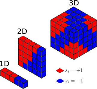
According to the third law of thermodynamics, the entropy of a perfect crystal must be 0 at 0 K. Working backwards from the third law and equation 6, magnetisation for a 3D Ising lattice can be calculated at 0K. For entropy to be 0, the multiplicity must equal 1. Hence, all spin states must be equivalent. Therefore magnetisation can take two values, of different sign, but same magnitude. For a 3D Ising lattice with 1,000 spin states, magnetisation can either take on a value of 1,000 or -1,000.
JC: Since magnetisation can take two values, the multiplicity of the ground state is 2, there is some residual entropy.
Energy and Magnetisation
Energy
Ising lattice energy was calculated in two different ways. One approach considered unique types of interaction; for example, all of the interactions that occur to the left of a point in the lattice, which included loops and if statements to ensure the correct equation is applied. Below is the code that calculated energy in this manner.
	    def energy(self):

		self.stored_energy = 0.0    #Need to define the variable that stores the total energy of the Ising lattice

		for i in range (self.n_rows):    #Looping function goes over each row
			for j in range (self.n_cols):    #Second looping function goes over each column

				#Two equations below are for interactions to the left
				if j > 0:	#Ensures that the column is energy can be calculated with the equation below
					self.stored_energy += -0.5*(self.lattice[i, j]*self.lattice[i, j - 1])
				else:    #Considers when it is the left column
					self.stored_energy += -0.5*(self.lattice[i, j]*self.lattice[i, -1])

				#Two equations below are for interactions to the right
				if j < self.n_cols-1:    #Ensures that the column is not on the right hand side before calculating energy
					self.stored_energy += -0.5*(self.lattice[i, j]*self.lattice[i, j + 1])
				else:    #Calculate energy fro the right hand side
					self.stored_energy += -0.5*(self.lattice[i, j]*self.lattice[i, 0])

				#Two equations below are for interactions above
				if i > 0:    #Defines energy calculation when the top row is not being considered
					self.stored_energy += -0.5*(self.lattice[i, j]*self.lattice[i - 1, j])
				else:    #Energy calculation for the top row
					self.stored_energy += -0.5*(self.lattice[i, j]*self.lattice[-1, j])

				#Two equations below are for interactions below
				if i < self.n_rows-1:    #For all rows apart from the bottom, the energy should be calculated in the following way
					self.stored_energy += -0.5*(self.lattice[i, j]*self.lattice[i+1 ,j])
				else:    #Energy calculation for when the bottom row is sampled
					self.stored_energy += -0.5*(self.lattice[i, j]*self.lattice[0, j])

		return self.stored_energy
This method involved including two equations for each interaction between spins, which arose because of the boundary conditions and limited size of the Ising lattice. Another method involved a larger lattice (3x3 randomly generated Ising lattices), which did not require each type of interaction to be specified, let alone two equations being required for each interaction. Only one equation for calculating energy was required. Alterations to the __init__ function and ILcheck.py were implemented, alongside defining a new function, TripleTransform. The implemented code is displayed below. Changes to the ILcheck.py file ensured the correct lattice size was plotted.
	def __init__(self, n_rows, n_cols):

		self.n_rows = n_rows
		self.n_cols = n_cols

		self.little_lattice = np.random.choice([-1, 1], size=(self.n_rows, n_cols)) 	#Generates self.n_rows*n_cols of -1 and +1, which is used for spin states

		self.lattice = TripleTransform(self.little_lattice) 	#Creates a 3x3 lattice of the randomly generated Ising  lattice

	def energy(self):
		self.stored_energy = 0.0

		for i in range(self.n_rows):   #First loop considers all rows
			o = self.n_rows + i    #Define a new variable that allows the center Ising lattice to be sampled
			for j in range(self.n_cols):    #Second loop defined for columns
				k = self.n_cols + j    #Second variable defined so middle Ising lattice is only considered
				self.stored_energy += - (self.lattice[o,k]/2)*(self.lattice[o + 1, k] + self.lattice[o - 1 ,k] + self.lattice[o, k + 1] + self.lattice[o, k - 1])
                                #Above is the formula to calculate energy for each spin

		return self.stored_energy

def TripleTransform(little_lattice):
	return np.array([row*3 for row in little_lattice.tolist()]*3) 	#Function that defines how to create larger 3x3 lattice
Owing to the boundary conditions of the Ising lattice, where spin states are taken in the Ising lattice does not matter. In the center of this large Ising lattice resides the original lattice; this lattice was chosen to determine the energy, as seen by the new variables (o and k) specified after each for loop.
JC: Your first energy function is correct and well commented. You don't actually need the i>0 or j>0 if statements, but this is a minor point. You have over complicated the question in the second energy function and while the second energy code will work to calculate the energy of the random lattice that you generate initially, it will not work properly during the Monte Carlo simulation as it will not pick up spin flips outside the central ninth of the lattice. Which of these codes did you use?
Magnetisation
As described previously, magnetisation can be calculated by taking the sum of all spin states. This was achieved by looping over each row and extracting spin values in each column with another loop; these values were added to a running total of the total spin. The code used is displayed below.
	def magnetisation(self):    #Function takes self, owing to variables being defined previously
		TS = 0    #Total spin of Ising self.lattice
		for i in range(self.n_rows):    #First loop that extracts defines what row
			for j in range(self.n_cols):    #Second loop that defines column
				TS += self.little_lattice[i, j]    #Adding spin state in i,j to TS
		return TS
JC: Code is correct and clearly commented.
Check
Energy and magnetisation checks for all of these codes were performed and found to agree with the expected values. Figure 2 displays the output from one of these calculations.
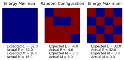
From inspection of equation 5, it would be expected that the minimum in energy would be -32.0, which can be seen in the subplot on the left hand side of figure 2. A maximum in magnetisation was also of the expected and can also be seen in this subplot. It was noted earlier that a maximum in energy would be reached when a checkers board arrangement of spins was established; the right hand side of figure 2 displays such a system. As discussed previously, the energy should equal that of equation 5, but with the opposite sign; equation 15 displays the result.
(15)
From equation 15, it can be concluded that the energy obtained from the maximum energy is, in fact, the result expected. Owing to equal numbers of each sign in this system, it would be expected that the magnetisation is zero, which can be seen in figure 2.
A randomly generated lattice should have energy and magnetisation values that are between the minimum and maximum already seen. Figure 2 displays results for the energy and magnetisation of a randomly generated lattice, which are, in fact, between the minimum and maximum values for energy and magnetisation.
JC: Well done for checking that the results make sense theoretically as well as using the ILcheck.py script.
Monte Carlo Simulation
Magnetisation Time Calculation
A system of N distinguishable spins, with n possible states, has a number of configurations given by equation 16; where , and are the number of configurations, number of states and number of spins, respectively.
(16)
Substituting the values provided yields configurations. From the assumption provided in the script, the time taken to perform these calculations can readily be calculated, which was found to have a time of s. Through dividing by the number of seconds in a minute, number of minutes in a hour, number of hours in a day and days in a year, the number of years taken to perform the calculation can be obtained, which yielded a value of years. This is a longer time period than what is thought to have passed in the universe. Hence, this is why the Monte Carlo function is employed.
JC: Putting the time into context, in terms of the age of the universe is a good idea.
Monte Carlo Function
The code written for the Monte Carlo function is displayed below.
def montecarlostep(self, T):

		if self.n_cycles == 0:    #Need to define the initial energy and magnetisation

			self.first_stored_energy = self.energy()    #Defining initial energy
			self.first_stored_magnetisation = self.magnetisation()    #Defining finial magnetisation

		random_i = np.random.choice(range(self.n_rows))    #Generates a random number between 0 and n_rows
		random_j = np.random.choice(range(self.n_cols))    #Generates a random number between 0 and n_cols
		self.lattice[random_i, random_j] = -1.0*self.lattice[random_i, random_j]    #A spin is selected using the random numbers generated previously
		self.second_stored_energy = self.energy()    #Energy of the new Ising lattice is calculated
		self.second_stored_magnetisation = self.magnetisation()    #Magnetisation is then calculated for the new Ising lattice
		self.delta_energy = self.second_stored_energy - self.first_stored_energy    #The difference between the fist and second energy is calculated to
                                                                                                                                          #see if the spin that has been flipped should be accepted

		if self.delta_energy < 0: #The new conditions are accepted in the following lines
			self.first_stored_energy = self.second_stored_energy
			self.first_stored_magnetisation = self.second_stored_magnetisation

		else:
			random_number = np.random.random()    #Generates random number
			self.exp_energy = exp(-(self.delta_energy)/(T))    #Calculating energy expression

			if random_number <= self.exp_energy:    #Condition for Monte Carlo simulation accepting change in spin
				self.first_stored_energy = self.second_stored_energy
				self.first_stored_magnetisation = self.second_stored_magnetisation
			else:    #Need to reject change if condition is not met
				self.lattice[random_i, random_j] = -1.0*self.lattice[random_i, random_j]
		self.n_cycles += 1
		self.E += self.first_stored_energy
		self.E2 += self.first_stored_energy*self.first_stored_energy
		self.M += self.first_stored_magnetisation
		self.M2 += self.first_stored_magnetisation*self.first_stored_magnetisation

		return self.first_stored_energy, self.first_stored_magnetisation
Changes to ILanim.py were also implemented so the algorithm would stop after a specified number of steps. Line 36 contained: “while true:”. As there was no condition for the boolean to change, calculations were perpetually performed. Hence, the line was altered to “while t < 950:”, which ensured that 950 iterations of the Monte Carlo algorithm were performed. This allowed the statistics function to execute, which permitted averages to be obtained.
JC: The Monte Carlo code looks good. You should have also included the statistics() function.
Expectation
The Curie temperature () is the temperature at which a material changes from its permanent magnetic state to being paramagnetic; for temperatures lower the material is a permanent magnet. Hence, if then it would be expected that spontaneous magnetisation occurs.
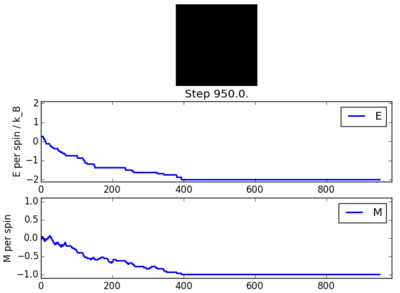
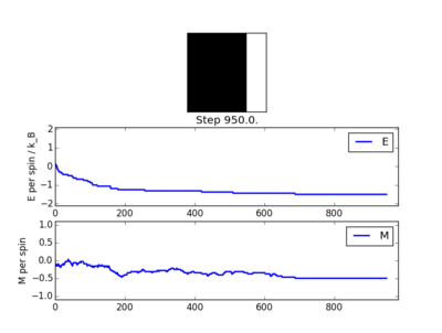
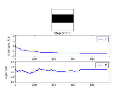
A temperature of 0.5 was initially taken. Several different results were obtained from this temperature. The majority of the time, spontaneous magnetisation would occur. However, in a few instances, a equilibrium state would be reached with bands of spins of the same sign. Figures 3 through 6 display some of the results obtained from calculations at a temperature of 0.5.
Figure 3 and 4 display examples where spontaneous complete magnetisation occurred. Whereas, figures 5 and 6 display partial magnetisation. It is known that, for a 2D Ising lattice, from the exact solution, that the Curie temperature should be at roughly 2.27. Hence, it would be expected that each calculation performed resulted in complete spontaneous magnetisation. This indicated that bands of different spin must arise from the small lattice size, not from temperature.
JC: These states with bands of different spins are metastable states. Did you run either of these for more steps? Eventually the ground state configuration should be found.
Outputs from the statistical function were also obtained from these calculations. Table 1 displays the results obtained from lattices displayed in figures 3 through 6.
| Figure | ||||
|---|---|---|---|---|
| 3 | ||||
| 4 | ||||
| 5 | ||||
| 6 |
It can be seen from table 1 that the energy values were not what would be expected from the minimum energy. An expected energy equation, per spin, can be obtained from dividing equation 5 by . Thus, a reduced energy per spin of -2 is expected. Owing to the fact that energy values have been taken from all steps in the Mote Carlo algorithm, it would be expected that an energy more positive than the minimum would be obtained. This is the case for all of the variables obtained from the statistics function.
Accelerating Code
Replacements for the energy and magnetisation functions can be seen below.
	def energy(self):

		self.stored_energy = 0.0

		self.stored_energy = -1.0*np.sum(np.multiply(self.lattice, np.roll(self.lattice, 1, 0)))
		self.stored_energy -= 1.0*np.sum(np.multiply(self.lattice, np.roll(self.lattice, 1, 1)))

		return self.stored_energy

	def magnetisation(self):
		TS = 0.0
		TS = 1.0*np.sum(self.lattice)
		return TS
Both energy and magnetisation functions were optimised by utilising numpy module functions. These changes eliminated the need for loops to be incorporated into the script, which are not always the most efficient ways to sum over arrays. The code could have also been accelerated by writing the critical code, that being the slow loop, in C++, which is a significantly faster programming language at performing iterative processes. In the last section of the report more detail is provided on this problem.
Two lines replaced the five previously used to calculate energy. These two new lines are essentially equivalent, with the only differences between them being the types of interaction they account for. Both lines contain a numpy sum module that requires at least one argument: an array of elements to sums over. Inside the sum function there is another numpy function, namely multiply. This requires at least two arguments which it multiples together element-wise. These arguments are the lattice and the final numpy module. Roll ensures that multiplication occurs with an element of the neighbour in the lattice, and that, when the index exceeds the size of the lattice, the first element of the matrix is taken instead. Three arguments have been specified for the numpy roll function: input array, which has taken the value of the lattice; shift, which is 1, owing to the neighbour of the lattice being required; and axis, which has been taken as 0 and 1 for neighbours above and to the right of the spin being considered, respectively. Therefore, an array is produced from multiplying neighbouring spins and is summed over to yield energy.
Calculating magnetisation is simply achieved with the numpy sum function, with the one argument being the randomly generated Ising lattice.
Table 2 was populated from running ILtimetrial.py with the different methods for calculating energy and magnetisation.
| Method | Mean | Standard Deviation |
|---|---|---|
| Orignial | ||
| Optimised |
Clearly, from table 2, the time taken for the optimised code for determining energy and magnetisation values was significantly lower than the original code. Furthermore, there was significantly less error associated to the time taken to perform these calculations, which indicates that there was less variation in the number of process performed.
Effect of Temperature
Modified Code
Below contains the modified Monte Carlo function and statistics function which permitted averages to be obtained after equilibrium was reached. Before the __init__ function a new variable was created, rn_cycles, which recorded the number of cycles that were performed after equilibrium was reached.
def montecarlostep(self, T):

		if self.n_cycles == 0:

			self.first_stored_energy = self.energy()
			self.first_stored_magnetisation = self.magnetisation()

		random_i = np.random.choice(range(self.n_rows))
		random_j = np.random.choice(range(self.n_cols))
		self.lattice[random_i, random_j] = -1.0*self.lattice[random_i, random_j]
                self.second_stored_energy = self.energy()
                self.second_stored_magnetisation = self.magnetisation()
                self.delta_energy = self.second_stored_energy - self.first_stored_energy

		if self.delta_energy < 0:
			self.first_stored_energy = self.second_stored_energy
			self.first_stored_magnetisation = self.second_stored_magnetisation

		else:
			random_number = np.random.random()
			self.exp_energy = exp(-(self.delta_energy)/(T))

			if random_number <= self.exp_energy:
				self.first_stored_energy = self.second_stored_energy
				self.first_stored_magnetisation = self.second_stored_magnetisation
			else:
				self.lattice[random_i, random_j] = -1.0*self.lattice[random_i, random_j]

		self.n_cycles += 1

		if self.n_cycles > 150000:    #Only values after the 150000 cycle contribute to the averages

			self.E += self.first_stored_energy
			self.E2 += self.first_stored_energy*self.first_stored_energy
			self.M += self.first_stored_magnetisation
			self.M2 += self.first_stored_magnetisation*self.first_stored_magnetisation
			self.rn_cycles +=1    #A new variable needed to be assigned to count the number of values recorded for averages

		return self.first_stored_energy, self.first_stored_magnetisation


	def statistics(self):    #n_cycles was removed and replaced with the new variable for all parameters
		self.AE = self.E/self.rn_cycles
		self.AE2 = self.E2/self.rn_cycles
		self.AM = self.M/self.rn_cycles
		self.AM2 = self.M2/self.rn_cycles

		return self.AE, self.AE2, self.AM, self.AM2
From inspection of figures 3 through 6, it can be seen that a 8x8 lattice takes no more than 800 cycles for equilibrium to be reached, provided complete spontaneous magnetisation occurred. Hence, averages could have been produced from cycles after the 2000th to ensure that the system had definitely equilibrated. However, this was not the largest Ising lattice used; a 32x32 lattice was the largest required lattice, which would require more steps in the Monte Carlo algorithm to equilibrate than a 8x8, owing to the larger number of spins that must be flipped. Figure 7 displays a graph produced from running ILfinalframe.py file with a reduced temperature of 0.25, lattice size of 32x32 and 200000 cycles. Clearly, from figure 7, it can be seen that spontaneous magnetisation occurred within this number of cycles, with equilibration occurring between 100000 and 150000 steps. Therefore, parameters shall be appended after 150000 to ensure that equilibration has occurred. For smaller lattices, this number of steps will not be required, but to keep the parameters of this computational exercise constant, they shall also be performed with this number of steps.
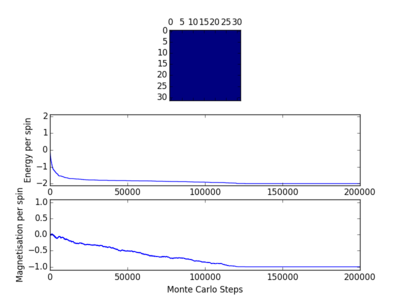
In some instances, even for this large number of steps, as seen in figure 8, complete spontaneous magnetisation did not occur. This suggests that a number of Monte Carlo simulations should be performed and averages of the averages should be attained. As this would be a difficult loop to incorporate and would result in a significantly longer running time, this change was not implemented.
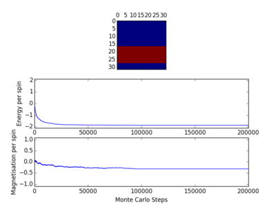
Table 3, seen below, displays the obtained results from simulations that had complete spontaneous magnetisation from identical initial conditions to that in figure 8. Therefore, it can be concluded that taking averages of parameters after 150000 cycles for 50000 cycles after yields representative results of the expected. Taking a large number of cycles after, of course, should produce values that are almost exactly of what is expected. Random fluctuations arise because of spin flips being accepted from random numbers, which result in mean values of energy being slightly higher than the expected.
| End State | ||||
|---|---|---|---|---|
| Blue | ||||
| Blue |
JC: Number of steps used for cutoff has been well justified and implemented energy and statistics code.
Range of Temperatures
An analytical solution of the 2D Ising lattice was solved by Lars Onsager in 1944. For square isotropic Ising lattices (where coupling in vertical direction is equal to that in horizontal) the analytical solution for magnetism, below the Curie temperature, and internal energy are given by equations 17 and 18, respectively; where , and can be seen in equation 19 and 20, respectively.
JC: Give the reference for where you found these equations and for Onsager's original paper.
(17)
(18)
(19)
(20)
Plotting energies and magnetisation obtained from the Monte Carlo simulation allowed a comparison to be made. Prediction of heat capacity can also be achieved from equation 18. Magnetic susceptibility can be predicted from equation 17.
A range of temperatures was produced from a np.arrange() function, which produces a range of values, of equal spacing, between two specified temperatures. The lower and upper limit, as specified, were set to 0.25 and upper 5.0625, respectively; a spacing of 0.0625 was chosen. This increment was chosen after analysis of heat capacity as a function of temperature revealed that information was lost about the true curvature if larger spaces were used.
Below displays the code used to investigate changes in energy and magnetisation as a function of temperature.
from IsingLattice import *
from matplotlib import pylab as pl
import numpy as np
import math as math

#The lines above import the required models
#Below specifies lattice size and then generates it

n_rows = 8
n_cols = 8
il = IsingLattice(n_rows, n_cols)
il.lattice = np.ones((n_rows, n_cols))
spins = n_rows*n_cols

runtime = 20000	#Number of steps are specified
times = range(runtime)	#A list is created to loop over

temps = np.arange(0.0625, 5.0625, 0.0625)	#Temperature ranges taken

#Empty arrays are prepared for collecting data in looping part

energies = []
magnetisations = []
energysq = []
magnetisationsq = []
EE = []
EM = []
PE= []
PM = []
PMT = []

for t in temps:   	#Loop over all temperatures, where t is the temperature
	for i in times:		#Loop for specified number of times
		energy, magnetisation = il.montecarlostep(t)		#Collect energy an magnetisation values from Monte Carlo algorithm
	aveE, aveE2, aveM, aveM2, n_cycles = il.statistics()	#Statistic values are obtained

	energies.append(aveE)	#Add energy value to array
	energysq.append(aveE2)	#Add energy squared to array
	magnetisations.append(aveM)	#Add magnetisation to array
	magnetisationsq.append(aveM2)	#Add magnetisation squared to array

	ee = math.sqrt(aveE2 - aveE*aveE)/spins	#Standard error per spin in energy
	em = math.sqrt(aveM2 - aveM*aveM)/spins	#Srandard error per spin in magnetisation
	EE.append(ee)	#Adding errors in energy to array
	EM.append(em)	#Adding errors in magnetisation to array

	if t < 2.2:	#Next part produces predicted magnetisation under Curie temperature

		pm = (1 - (math.sinh(2/t))**(-4))**(1/8)
		PM.append(pm)
		PMT.append(t)

	#Next section predicts energy

	k = (math.sinh(2/t)*math.sinh(2/t))**-1.0

	a = (math.tanh(2/t))**-1.0
	b = (2/math.pi)*(2*(math.tanh(2/t))**2-1)
	c = 4*k*(1 + k)**-2.0

	#Numpy module used to integrate function

	def intergrand(x, c):
		return (1.0 - c*(math.sin(x))**2)**(-0.5)

	I = integrate.quad(intergrand, 0, math.pi/2, args=(c))

	pe = - a*(1.0 + b*I[0])
	PE.append(pe)

	il.E = 0.0
	il.E2 = 0.0
	il.M = 0.0
	il.M2 = 0.0
	il.n_cycles = 0.0
	il.rn_cycles = 0.0

#Next section calculates energy and magnetisation values per spin

energy = np.array(energies)/spins
energy2 = np.array(energysq)/spins
mag = np.array(magnetisations)/spins
mag2 = np.array(magnetisationsq)/spins

#Next section plots energy and magnetisation as a function of temperature for Monte Carlo and analytical

fig = pl.figure()
enerax = fig.add_subplot(2,1,1)
enerax.set_ylabel("Energy per spin")
enerax.set_xlabel("Temperature")
enerax.set_ylim([-2.1, 2.1])
enerax.errorbar(temps, energy, yerr= EE)
magax = fig.add_subplot(2,1,2)
magax.set_ylabel("Magnetisation per spin")
magax.set_xlabel("Temperature")
magax.errorbar(temps, mag, yerr= EM)
magax.set_ylim([-1.1, 1.1])
enerax.plot(temps, np.array(energies)/spins, label = 'Monte Carlo')
enerax.plot(temps, PE, label = 'Predicted')
magax.plot(temps, np.array(magnetisations)/spins, label = 'Monte Carlo')
magax.plot(PMT, PM, label = 'Predicted')
pl.show()

final_data = np.column_stack((temps, energies, energysq, magnetisations, magnetisationsq))
np.savetxt("TR_" + str(n_rows) + "x" + str(n_rows) + ".dat", final_data)
JC: Great idea to compare the results with the analytical result, well done.
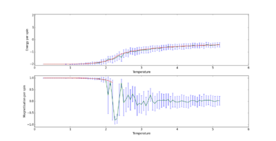
Figure 9 displays the output from ILtemperaturerange.py for a 8x8 lattice. It can be seen that energy and magnetisation reduces to zero as temperature increases, which was expected from the analytical solutions. For each flip in spin, there will always be the some change in energy, which is why the inequality in the Monte Carlo algorithm is not a less than or equal to. If there is not a negative change in energy, the Monte Carlo algorithm uses random numbers () and equation 21 to decide if the change in spin should be accepted. As temperature increases, the affect of this change in energy becomes smaller. Hence, the energy term tends to 1 as the expression in the exponential tends to larger values. This increases the probability that the random number is smaller than the exponential of the energy, which therefore, increases the probability that a change in spin will be accepted. For very large temperatures, almost all changes in spin shall be accepted. Thus, no spontaneous magnetisation occurred at high temperatures, which results in no ordering of the system and lowering of reduced energy; the system remains random.
(21)
Error bars were produced with the standard deviation of each parameter and included in figure 9. As there was a large sample size, the distribution of values was quite large. Another error calculation was performed, with the same lattice size, that took into account the sample size. Figure 10 displays the same calculation, but with error bars that correspond to the standard error, not standard deviation. Clearly, from this figure, the error is significantly smaller. As the standard error does not put the computationally obtained within that of the analytical, the standard error should not be used to determine error bars. Producing error bars with standard deviation ensures computationally calculated values from Monte Carlo simulations are in agreement with the exact solution, within error.
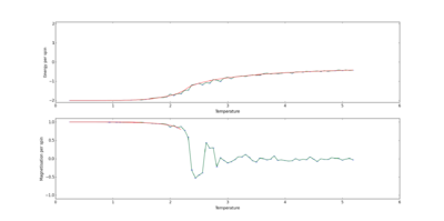
Mean values need to be obtained from running many Monte Carlo simulations instead of taking mean values of a large number of steps for the same simulation. Therefore, if the system does not equilibrate correctly, as seen in figures 5 and 6, there is a chance for correction. Performing averages in this manner would reduce the probability that a energy or magnetisation values is significantly different from the trend, which is seen for small lattice systems.
JC: Good consideration of the effect that metastable states will have on your results. You need to put a legend on your plot though so that it is clear what each line corresponds to.
Effect of System Size
It would expect that as the size of the system increases, there is less fluctuations in average values of energy and magnetisation, owing to an increase in statistical sample size. Furthermore, it would be expected that larger Ising lattices are closer to the analytical solution. Figure 11 displays energy as a function of temperature for lattice sizes from 2x2 to 64x64.
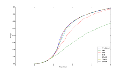
From figure 11 it can be seen that as lattice size increases, energy as a function of temperature tends to that predicted. Hence, as expected, larger lattice sizes produce more accurate results; they also produced slightly less fluctuations, which was also expected.
A lattice size of 8x8 is sufficient to capture long range fluctuations. This size was chosen because it has essentially identical points to larger lattice sizes; however, owing to its smaller size, it is less computationally expensive than that of other lattices. Smaller lattices, specifically 2x2 and 4x4, were unable to represent long range fluctuations in energy as a function of temperature. In both cases, energy was predicted to be more negative than larger lattices and analytical.
Energy per spin as a function of temperature was plotted for the provided C++ data and displayed in figure 12 for comparative purposes.
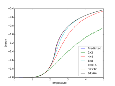
There is clearly better agreement between larger lattice sizes, more specifically for those above 16x16, and analytical than for data obtained from python. Furthermore, there is significantly less fluctuations in data compared to that obtained from python, which was also expected. Lattice sizes of 4x4 and 2x2 were still inadequate at describing how energy per spin changes as a function of temperature. Hence, it can be concluded that these lattice sizes fail to describe the analytical solution because of their size and not because of the number of iterations in the Monte Carlo function.
Figure 13 displays magnetisation per spin as a function of temperature for lattices seen in figure 11. As seen in the previous section, magnetisation decreases to zero as temperature increases.
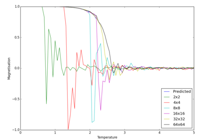
Similar expectations for different lattices sizes would also be expected for magnetisation per spin as they were for energy per spin, owing to their intrinsic link to spin states. Similarly, it can be seen that lattice sizes of 2x2 and 4x4 were erratic. This furthers the case that these lattice sizes can not be used to determine long range fluctuations. Lattices sizes of 8x8 and 16x16 produce representative descriptions of magnetisation per spin as a function of temperature. Once temperature approaches the Curie temperature, there is dramatic fluctuations in magnetisation, which would be expected, owing to the material loosing its permanent magnetic properties. However, if they are compared to the largest lattice size investigated, it can be seen that they fluctuations significantly more. Prediction of magnetisation of the 2D Ising lattice can only be performed up to the Curie temperature, and no further. Therefore, it can be concluded that a lattice size of 8x8 is sufficient in describing long range fluctuations in magnetisation up to the Curie temperature.
Smaller lattices, between 2x2 and 4x4, magnetisation per spin reduced to zero at temperatures lower than the Curie temperature when compared to that of larger lattices, such as 8x8 and above. This observation can be explained by considering how a change in one spin effects the whole lattice. For smaller lattices, changing one spin influences the whole lattice to a larger extent than that of a larger lattice. Hence, if by chance, which is an intrinsic part of the Monte Carlo simulation, changing one spin results in a knock on effect that results on magnetisation that can result in no spontaneous magnetisation occurring.
A plot of magnetisation per spin as a function of temperature was also produced for C++ data; figure 14 displays the results.
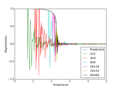
In a similar manner to energy per spin, magnetisation per spin has been predicted to a higher degree of accuracy for a larger system by C++ data. However, as prediction of magnetisation per spin can only be made up to, not beyond, the Curie temperature, there is less room for discussion of errors.
The code below was utilised to obtain these figures.
from matplotlib import pylab as pl
import numpy as np
import math as math
import scipy.integrate as integrate

#Modules required were imported

#LS = [2, 3, 4, 5, 6, 7, 8, 10, 12, 14, 16, 20, 24, 28, 32, 64]
LS = [2, 4, 8, 16, 32, 64] 	#Smaller set of data used for plotting
LLS = len(LS)

PE = []		#Empty array created to obtain predicted data
temps = np.arange(0.25, 5.0625, 0.0625)	#Temperature range created

for t in temps: 		#Predicted temperatures calculated for each temperature

	k = (math.sinh(2.0/t)*math.sinh(2/t))**-1.0

	a = (math.tanh(2.0/t))**-1.0
	b = (2.0/math.pi)*(2.0*(math.tanh(2/t))**2-1.0)
	c = 4*k*(1.0 + k)**-2.0

	def intergrand(x, c):
		return (1.0 - c*(math.sin(x))**2)**(-0.5)

	I = integrate.quad(intergrand, 0, math.pi/2, args=(c))

	pe = - a*(1.0 + b*I[0])

	PE.append(pe)	#Predicted data appended

pl.figure()

pl.plot(temps, PE, label = 'Predicted')		#Predicted data plotted

for i in range(LLS):	#Data files for each lattice size extracted

	spins = LS[i]*LS[i]	#Number of spins for each lattice size determined

	M_data = np.loadtxt('M_' + str(LS[i]) + 'x' + str(LS[i]) + '.dat')

	T = M_data[:,0]	#Temperatures obtained
	E = M_data[:,1]	#Energy obtained

	pl.plot(T, E/spins, label = str(LS[i]) + 'x' + str(LS[i]))
	pl.ylabel("Energy")
	pl.xlabel("Temperature")
	pl.legend(loc='lower right')

pl.show()

pl.figure()

PM = []		#Empty array for predicted magnetisation created
temps = np.arange(0.25, 2.25, 0.0625)	#Temperature range just below Curie created

for t in temps:		#Magnetisations predicted for each temperature
	pm = (1 - (math.sinh(2/t))**(-4))**(1/8)
	PM.append(pm)
pl.plot(temps, PM, label = 'Predicted')

for i in range(LLS):	#Data files imported to extract magnetisation for each lattice

	spins = LS[i]*LS[i]

	M_data = np.loadtxt('M_' + str(LS[i]) + 'x' + str(LS[i]) + '.dat')

	T = M_data[:,0]
	M = M_data[:,3]

	pl.plot(T, M/spins, label = str(LS[i]) + 'x' + str(LS[i]))
	pl.ylabel("Magnetisation")
	pl.xlabel("Temperature")
	pl.legend(loc='lower right')

pl.show()
JC: Again good use of analytical results and good, thorough analysis and comparison between different system sizes. 8x8 correctly identified as sufficient to capture most of the long range fluctuations.
Heat Capacity and Magnetic Susceptibility
Derivation
Starting from the statistical thermodynamic definition of internal energy, which can be seen in equation 22 (where and are the internal energy and probability of each energy, respectively), the heat capacity can be expressed in terms of obtainable energy values from calculations. Thus, prediction of the heat capacity can be achieved.
(22)
The probability of each energy state can be seen in equation 23; where is the partition function.
(23)
Heat capacity is defined in equation 24. Substituting equation 22 into 24 and taking the derivative with respect to temperature yields equation 25.
(24)
(25)
Equation 25 can be simplified to yield 26, which can then be compared to definitions for the mean internal energy and mean of the square of internal energy, which are displayed in equations 27 and 28, respectively. These mean values can be obtained from the statistical function in the code described above.
(26)
(27)
(28)
Hence, a simplification can be made; equation 29 displays the result.
(29)
JC: Clear derivation shows you have a good understanding of the theory.
Heat Capacity as a Function of Temperature
Figure 15 displays the output, for a 8x8 lattice, from a piece of code which was modified from the temperature range calculations to calculate heat capacity; the code for which can also be seen below.

Clearly, there is a maximum in heat capacity when the largest changes in energy occur, which is expected from the definition of heat capacity. Below displays modified code from ILtemperaturerange.py to calculate heat capacities for each lattice size.
from IsingLattice import *
from matplotlib import pylab as pl
import numpy as np

n_rows = 32
n_cols = 32
il = IsingLattice(n_rows, n_cols)
il.lattice = np.ones((n_rows, n_cols))
spins = n_rows*n_cols
runtime = 20000
times = range(runtime)
temps = np.arange(0.25, 5.0625, 0.0625)
energies = []
magnetisations = []
energysq = []
magnetisationsq = []
heatcapacity = []	#Empty array created for heat capacity
for t in temps:
    for i in times:
        energy, magnetisation = il.montecarlostep(t)
    aveE, aveE2, aveM, aveM2, n_cycles = il.statistics()
    energies.append(aveE)
    energysq.append(aveE2)
    magnetisations.append(aveM)
    magnetisationsq.append(aveM2)
    hc = (aveE2 - aveE*aveE)/(t*t)   	#Addition to calculate heat capacity
    heatcapacity.append(hc)	          #Heat capacity values appended to empty array
    #reset the IL object for the next cycle
    il.E = 0.0
    il.E2 = 0.0
    il.M = 0.0
    il.M2 = 0.0
    il.n_cycles = 0
    il.rn_cycles = 0

fig = pl.figure()
enerax = fig.add_subplot(3,1,1)
enerax.set_ylabel("Energy per spin")
enerax.set_xlabel("Temperature")
enerax.set_ylim([-2.1, 2.1])
magax = fig.add_subplot(3,1,2)
magax.set_ylabel("Magnetisation per spin")
magax.set_xlabel("Temperature")
magax.set_ylim([-1.1, 1.1])
heatc = fig.add_subplot(3,1,3)
heatc.set_ylabel("Heat capacity per spin")
heatc.set_xlabel("Temperature")
enerax.plot(temps, np.array(energies)/spins)
magax.plot(temps, np.array(magnetisations)/spins)
heatc.plot(temps, np.array(heatcapacity)/spins)
pl.show()

final_data = np.column_stack((temps, energies, energysq, magnetisations, magnetisationsq, heatcapacity))
np.savetxt("M_" + str(n_rows) + "x" + str(n_rows) + ".dat", final_data)
Prediction of heat capacity was achieved from taking the first derivative with respect to temperature of the analytical solution of the energy. Equation 18 and 24 display the analytical solution of energy per spin for a 2D Ising lattice and heat capacity, respectively.
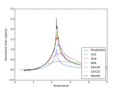
Figure 16 displays heat capacity as a function of temperature for lattice sizes from 2x2 to 64x64. This graph was produced by a modifying code utilised in the Effect of Lattice Size section and from the output files of the above code. It can be seen that there is relatively good agreement between computationally obtain values and analytical, which is seen in blue. As expected, larger lattice sizes produce heat capacities that resemble analytical more accurately than smaller ones.
JC: Nice clear graph to show the trend with system size.
It can be seen, from figure 16, that there is a maximum in heat capacity, for all lattice sizes, which resides around the Curie temperature, between temperatures of 2 and 3. At low temperatures, a maximum in heat capacity occurred because of the Schottky anomaly. This phenomena is explained from the fact that there is a finite number of energy levels. As temperature increases, energy levels become saturated, which causes excitation to become less likely. Hence, larger amounts of energy need to be supplied for an increase in temperature. There comes a point when energy absorbed by the system is infrequent, which causes essentially no increase in temperature, so the heat capacity reduces. For the specific case of a 2D Ising lattice, the explanation is slightly different. At low temperatures. not all change in spins are accepted, which causes there to be little change in energy, and therefore, a low heat capacity. For temperatures around the Curie temperature, a higher proportion of spins flips are accepted, so there is an increase in energy per spin, which causes the heat capacity to increase. Large temperatures, as described previously, result in almost all spin flips being accepted, which results in a random Ising lattice. This lattice has a roughly constant energy near zero, which causes there to be a low heat capacity.
JC: The peak in the heat capacity can also be explained in terms of the rate of change of entropy with temperature, since heat capacity can be written as . What should the heat capacity be analytically at the Curie temperature?
Each of these maximum points occurs at the Curie temperature, which is the temperature at which a material losses its permanent magnetic properties. At this point, energy needs to be supplied to flip electronic spin states. Thus, it might be expected that a maximum in heat capacity is observed.
The code used to produce figure 16 can be seen below.
from matplotlib import pylab as pl
import numpy as np
import math as math
import scipy.integrate as integrate

#LS = [2, 3, 4, 5, 6, 7, 8, 10, 12, 14, 16, 20, 24, 28, 32, 64]
LS = [2, 4, 8, 16, 32, 64]
LLS = len(LS)

PE = []
temps = np.arange(0.25, 5.0625, 0.0625)

for t in temps:

	k = (math.sinh(2/t)*math.sinh(2/t))**-1.0

	a = (math.tanh(2/t))**-1.0
	b = (2/math.pi)*(2*(math.tanh(2/t))**2-1)
	c = 4*k*(1 + k)**-2.0

	def intergrand(x, c):
		return (1.0 - c*(math.sin(x))**2)**(-0.5)

	I = integrate.quad(intergrand, 0, math.pi/2, args=(c))

	pe = - a*(1.0 + b*I[0])
	PE.append(pe)

DPET = []	#Empty array for derivative of predicted energy with respect to temperature

LT = len(temps) - 1	#Taking the approximate derivative requires one less temperature value

for u in range(LT): 	#Loop calculates derivative of predicted energy.

	dpet = (PE[u + 1] - PE[u])/0.0625
	DPET.append(dpet)

d_temps = np.delete(temps, LT)

DPET_M = np.max(DPET)	#Maximum in derivative of energy with respect to temperature found
NDPET = []	#Empty array for normalised values

for u in range(LT):	#Loop that calculated normalised values
	NDPET.append(DPET[u]/DPET_M)

pl.plot(d_temps, NDPET, label = 'Predicted')		#Normalised predicted values plotted

for i in range(LLS):

	spins = LS[i]*LS[i]

	M_data = np.loadtxt('C_' + str(LS[i]) + 'x' + str(LS[i]) + '.dat')

	T = M_data[:,0]
	HC = M_data[:,5]

	pl.plot(T, HC, label = str(LS[i]) + 'x' + str(LS[i]))
	pl.ylabel("Normalised Heat Capacity")
	pl.xlabel("Temperature")
	pl.legend(loc='lower right')

pl.show()
Magnetic susceptibility
Another physical parameter of a 2D Ising lattice is its magnetic susceptibility, which measures how a material responds to external magnetic fields. Equation 30 describes magnetic susceptibility, where is the magnetic susceptibility. Positive magnetic susceptibility values correspond to materials that can be paramagnetic and ferromagnetic, amongst other types (antiferromagnetic and ferrimagnetic). It is expected that, below the Curie temperate, the 2D Ising lattice is ferromagnetic and above paramagnetic.
(30)
Figure 17 displays the output from including magnetic susceptibility into the heat capacity calculations from the previous section on a 8x8 Ising lattice.
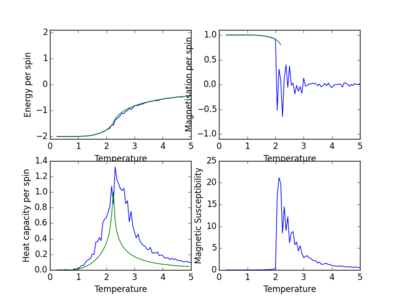
It can be seen that magnetic susceptibility is always positive, and that, after the Curie temperature, there is a large increase in magnetic susceptibility. Below the Curie temperature, it is expected that a material is ferromagnetic. Materials which have this type of magnetisation are not that susceptible to external magnetic fields. Hence, it would be expected that, below the Curie temperature, the magnetic susceptibility is lower than for temperatures larger.
JC: Good extension to look at magnetic susceptibility.
Curie Temperature
Comparison to C++
Figure 18 displays the output from the comparison between python and C++ for a 8x8 Ising lattice. Clearly, there are less fluctuations in energy, magnetisation and heat capacity from data obtained from C++ data when compared to python.
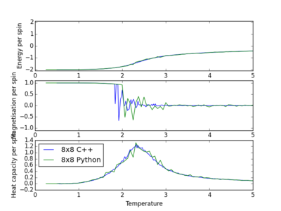
A generic script was produced that could plot all data sets, or a specific subset, for energy per spin, magnetisation per spin and heat capacity together on a single graph. Below is the code which was written for this plotting. No comments are included as it is essentially the same as previous examples.
from matplotlib import pylab as pl
import numpy as np

#LS = [2, 3, 4, 5, 6, 7, 8, 10, 12, 14, 16, 20, 24, 28, 32, 64]
#LS = [2, 4, 8, 16, 32, 64]
LS = [8]
LLS = len(LS)

fig = pl.figure()

for i in range(LLS):

	spins = LS[i]*LS[i]

	C_data = np.loadtxt('C_' + str(LS[i]) + 'x' + str(LS[i]) + '.dat')

	C_T = C_data[:,0]
	C_E = C_data[:,1]
	C_M = C_data[:,3]
	C_C = C_data[:,5]

	M_data = np.loadtxt('M_' + str(LS[i]) + 'x' + str(LS[i]) + '.dat')

	M_T = M_data[:,0]
	M_E = M_data[:,1]
	M_M = M_data[:,3]
	M_C = M_data[:,5]

	enerax = fig.add_subplot(3 ,1, 1)
	enerax.set_ylabel("Energy per spin")
	enerax.set_xlabel("Temperature")
	enerax.set_ylim([-2.1, 2.1])

	magax = fig.add_subplot(3, 1, 2)
	magax.set_ylabel("Magnetisation per spin")
	magax.set_xlabel("Temperature")
	magax.set_ylim([-1.1, 1.1])

	heatc = fig.add_subplot(3, 1, 3)
	heatc.set_ylabel("Heat capacity per spin")
	heatc.set_xlabel("Temperature")

	enerax.plot(C_T, C_E, label = str(LS[i]) + 'x' + str(LS[i]) + ' C++')
	magax.plot(C_T, C_M, label = str(LS[i]) + 'x' + str(LS[i]) + ' C++')
	heatc.plot(C_T, C_C, label = str(LS[i]) + 'x' + str(LS[i]) + ' C++')

	enerax.plot(M_T, M_E/spins, label = str(LS[i]) + 'x' + str(LS[i]) + ' Python')
	magax.plot(M_T, M_M/spins, label = str(LS[i]) + 'x' + str(LS[i]) + ' Python')
	heatc.plot(M_T, M_C/spins, label = str(LS[i]) + 'x' + str(LS[i]) + ' Python')
	pl.legend(loc= 'upper left')

pl.show()
Polynomial Fit
A python script for fitting a polynomial to the obtained data is attached below. The degree of polynomial fitted could easily be adjusted by inserting a different number into np.polyfit() function.
from matplotlib import pylab as pl
import numpy as np
from pylab import *
from scipy.optimize import curve_fit

#Above imports all of the required modules for the script

#LS = [2, 3, 4, 5, 6, 7, 8, 10, 12, 14, 16, 20, 24, 28, 32, 40, 48, 56, 64]	#If required, a larger number of data files could be sampled
LS = [2, 4, 8, 16, 32, 64]	#Defining the specified lattices
LLS = len(LS)	#Defining the number of lattices used

CT = []		#An empty list was created to obtain Curie temperatures

for i in range(LLS):	#Loop goes over all lattices defined

	M_data = np.loadtxt('M_' + str(LS[i]) + 'x' + str(LS[i]) + '.dat')	#Generic expression imports required data file for lattice

	T = M_data[:, 0]	#Extract required temperatures from data file
	C = M_data[:, 5]	#Extract required heat capacities from data file
	Cmaxi = np.max(C)	#Maximum heat capacity was found
	Tmaxi = T[C == Cmaxi]	#Temperature at maximum heat capacity found

	fit = np.polyfit(T, C, 10)		#Fit a tenth order polynomial

	T_min = np.min(T)	#Minimum temperature found
	T_max = np.max(T)	#Maximum temperature found
	T_range = np.linspace(T_min, T_max, 1000) 	#A set of temperates, between the minimum and maximum, defined in the previous two lines, was produced
	fitted_C_values = np.polyval(fit, T_range) 	#Corresponding values of heat capacity generated from temperature range and fitted polynomial
	Cmaximum = np.max(fitted_C_values)	#Maximum in generated heat capacity found
	Tmaximum = T_range[fitted_C_values == Cmaximum]	#Temperature at maximum heat capacity found, which is also known as Curie temperature

	#Range about maximum defined in next two lines
	Tmin = Tmaxi - 1 #Lower temperature set to maximum temperature minus 1
	Tmax = Tmaxi + 1 #Upper temperature set to maximum temperature plus 1

	selection = np.logical_and(T > Tmin, T < Tmax) #Choosing indexes for temperature values in range specified
	peak_T_values = T[selection]		#Producing an array of the specified temperature values
	peak_C_values = C[selection]	#Producing array of heat capacities
	peak_T_range = np.linspace(Tmin, Tmax, 1000)  	#Next lines repeats
	peak_fit = np.polyfit(peak_T_values, peak_C_values, 4)
	peak_fitted_C_values = np.polyval(peak_fit, peak_T_range)
	C_maximum = np.max(peak_fitted_C_values)
	T_maximum = peak_T_range[peak_fitted_C_values == C_maximum]

	CT.append(float(T_maximum))	#Adding the obtained Curie temperature to array

	#Following lines plot the obtained data and polynomial fits with a legend
	pl.figure()
	pl.plot(T, C, label = 'Data')
	pl.plot(T_range, fitted_C_values, label = 'Fitted data')
	pl.plot(peak_T_range, peak_fitted_C_values, label = 'Peak fitted data')
	pl.scatter(Tmaximum, Cmaximum, marker="o")
	pl.scatter(T_maximum, C_maximum, marker="o")
	pl.ylabel("Heat capacity per spin")
	pl.xlabel("Temperature")
	pl.legend(loc='upper left')
	pl.show()

#File is created
final_data = np.column_stack((LS, CT))
np.savetxt("CT.dat", final_data)
JC: Polyfit and polyval functions used correctly.
A range of data was chosen equidistant from the maximum heat capacity value to allow a range to be specified generally for each case. Above, it can also be seen that the script would produce a polynomial fit for the whole data set and subset about the maximum for each lattice before plotting the Curie temperature as a function of lattice size.
A for loop was added to allow quick plotting of a number of different degrees of polynomial for both peak data and the whole range; the relevant code for which can be seen in the following two sections, respectively.
pd = [2,4,6,8]
	lpd = len(pd)

	pl.figure()

	for j in range(lpd):

		selection = np.logical_and(T > Tmin, T < Tmax)
		peak_T_values = T[selection]
		peak_C_values = C[selection]
		peak_T_range = np.linspace(Tmin, Tmax, 1000)
		peak_fit = np.polyfit(peak_T_values, peak_C_values, pd[j])
		peak_fitted_C_values = np.polyval(peak_fit, peak_T_range)
		C_maximum = np.max(peak_fitted_C_values)
		T_maximum = peak_T_range[peak_fitted_C_values == C_maximum]

		CT.append(float(T_maximum))


		pl.plot(peak_T_range, peak_fitted_C_values, label = 'Peak fitted data with ' + str(pd[j]) +' order poylnomial')
		pl.scatter(T_maximum, C_maximum, marker="o")

	pl.plot(T, C, label = 'Data')
	pl.plot(T_range, fitted_C_values, label = 'Fitted data')
	pl.scatter(Tmaximum, Cmaximum, marker="o")
	pl.ylabel("Heat capacity per spin")
	pl.xlabel("Temperature")
	pl.legend(loc='lower right')
	pl.show()
pl.figure()

	for j in range(lpd):
		#first we fit the polynomial to the data
		fit = np.polyfit(T, C, pd[j]) # fit a third order polynomial

		#now we generate interpolated values of the fitted polynomial over the range of our function
		T_min = np.min(T)
		T_max = np.max(T)
		T_range = np.linspace(T_min, T_max, 1000) #generate 1000 evenly spaced points between T_min and T_max
		fitted_C_values = np.polyval(fit, T_range) # use the fit object to generate the corresponding values of C
		Cmaximum = np.max(fitted_C_values)
		Tmaximum = T_range[fitted_C_values == Cmaximum]
		pl.plot(T_range, fitted_C_values, label = 'Fitted data ' + str(pd[j]) +' order polynomial')
		pl.scatter(Tmaximum, Cmaximum, marker="o")

	Tmin = Tmaxi - 1 #for example
	Tmax = Tmaxi + 1 #for example

	selection = np.logical_and(T > Tmin, T < Tmax) #choose only those rows where both conditions are true
	peak_T_values = T[selection]
	peak_C_values = C[selection]
	peak_T_range = np.linspace(Tmin, Tmax, 1000)
	peak_fit = np.polyfit(peak_T_values, peak_C_values, 4)
	peak_fitted_C_values = np.polyval(peak_fit, peak_T_range)
	C_maximum = np.max(peak_fitted_C_values)
	T_maximum = peak_T_range[peak_fitted_C_values == C_maximum]

	CT.append(float(T_maximum))

	pl.plot(peak_T_range, peak_fitted_C_values, label = 'Peak fitted data with 4 order poylnomial')
	pl.scatter(T_maximum, C_maximum, marker="o")
	pl.plot(T, C, label = 'Data')
	pl.ylabel("Heat capacity per spin")
	pl.xlabel("Temperature")
	pl.legend(loc='lower right')
	pl.show()
It was found that a fourth and tenth order polynomial was sufficient to describe heat capacity as a function of temperature for the peak range of data and full range, respectively. In addition, it was also found that, for smaller lattice sizes, smaller orders of polynomial were able to adequately describe the variation in heat capacity with temperature. Hence, why the orders were chosen for the largest lattice size, not the smallest. Figure 19 displays the results obtained from performing the calculations on a 8x8 Ising lattice.
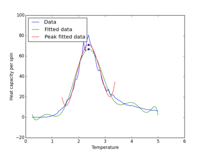
Clearly, by taking a smaller range of data, the fitting process is optimised. A smaller number of points needs to be sampled and a polynomial with a smaller order is required to represent the computationally obtained. Both of these processes require computational time, and so, by removing them, the time taken to execute this part pf the script was reduced.
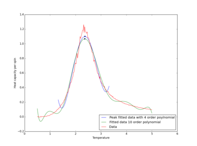
The plotting was also repeated for the provided C++ data, which can be seen in figure 20. It was noticed that higher order polynomials were required for C++ data than python. The reason for this being an increased peak height and reduction in width, which was caused by the larger change in energy observed for C++ data at the Curie temperature.
Heat Capacity Maximum
The scaling relationship, which can be seen in equation 31, predicts what the Curie temperature should be for different lattice sizes. Smaller lattice sizes are expected to have larger Curie temperatures because of their more negative energies at temperature about, and larger than, the Curie temperature. Discussion of why they are more negative can be seen in a previous section.
(31)
Modification of the previous script was performed to allow the Curie temperature to be obtained at an infinite lattice size. Below is the addition that was made.
def func(LS, a, b):	#A function was defined that would output the scaling relation
    return a/LS + b	#Equation for scaling relation

popt, pcov = curve_fit(func, LS, CT)	  #Curve fit scaling relation

LSL = linspace(2, 64, 1000)		#Range of lattice sixes created for smooth plot

#Figure plots actual data with fitted

pl.figure()
pl.plot(LS, CT)
pl.plot(LSL, func(LSL,*popt))
pl.ylabel("Curie temperature")
pl.xlabel("Lattice size")
pl.show()

print('A and T,C,infinity are given by ' + str(popt[0]) + ' and ' + str(popt[1]) + ‘, respectively.')
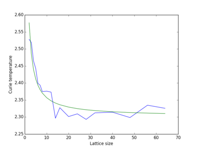
Figure 21 displays the results obtained from a large number of lattices, which can be seen at the top of the code from Polynomial Fit. It is evident that, as the lattice size increases, there is a reduction in Curie temperature, which is expected from equation 31. From the analytical solution of the Ising lattice, the Curie temperature can be predicted; equation 32 displays this result.
(32)
Hence, it is evident that there is good agreement between analytical and computational obtain, owing to the fact that a Curie temperature of 2.31 was obtained form computational.
JC: Why did you choose to plot the Curie temperature against L and fit to a curve to obtain T infinity? What about plotting Curie temperature against 1/L, fitting to a straight line and reporting the intercept?
Prediction of the lattice size that produced a 1% error can be achieved from equation 31 and the coefficients that were calculated from the script; where and were found to be 0.40 and 2.31, respectively. It was found that a lattice size of 18x18 would be sufficient to this degree of accuracy.
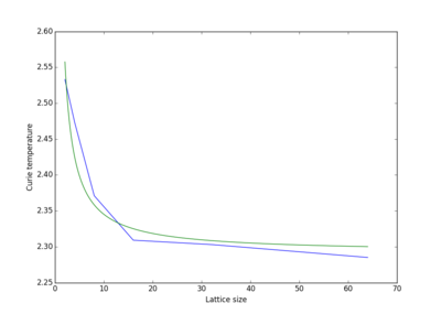
Figure 22 displays Curie temperature as a function of lattice size for the provided C++ data. It can be seen that a similar fit is achieved. However, as seen before, and expected, there is less deviation of computationally obtained from the fitted. The Curie temperature at an infinite lattice size was found to be 2.29, which is slightly better than that obtained from python.
Sources of error included: when equilibration is decided; if the system equilibrates; and number of steps used to average parameters. Owing to the fact that the number of steps taken from equilibration to be reached was calibrated to a 32x32 lattice system, all lattices smaller than this one would have definitely equilibrated to some state before parameters were collected for statistics. Therefore, the number of steps chosen before equilibration should not have resulted in an error for lattices smaller than 32x32, and would have produced a small error for the 64x64 lattice. Furthermore, there would have been very little contribution to the error from the number of values obtained for each parameter for the statistics. Each parameter had 50,000 values for each parameter, which should have been sufficient it averaging random fluctuations in the equilibrated system. Sometimes the Monte Carlo simulation would not equilibrate to the global minimum, but would equilibrate to a local minimum, as seen in figures 5 and6. These systems did not have the correct energy and magnetisation values that was expected, and therefore, caused significant alterations to these values produced by the statistics function. Equilibration to local minimums was likely to cause the most significant error in the simulation.
JC: What about errors introduced by the fitting?


