Talk:Mod:YR3CMPRM1412

The Ising Model

Introduction

The Ising model, formulated in 1920 by Wilhelm Lenz, is a lattice model and the simplest mathematical description of ferromagnetic materials. Ising first used the model to study ferromagnetism but it has since been used to model other systems that exhibit co-operative phenomena and examples of systems studied thus far include surfaces of separation at phase boundaries and gas-liquid systems at their critical point. For this experiment, the Ising model will be used to study ferromagnetic materials.

Calculating the interaction energy and net magnetisation for example lattices

Task 1

In the lowest energy configuration of an Ising lattice in D dimensions all spins are aligned and each spin is interacting with 2*D spins in adjacent cells. For a lattice with N spins, the energy of its lowest energy configuration can be written in terms of D and N by noting that the total number of interactions is:

$$\begin{gathered} \sum _i^N\sum _{j \\ \in \\ \mathrm{n}\mathrm{e}\mathrm{i}\mathrm{g}\mathrm{h}\mathrm{b}\mathrm{o}\mathrm{u}\mathrm{r}\mathrm{s}\left(i\right)}{s}_i{s}_j=2DN \end{gathered}$$

and substituting this expression into the original equation for the interaction energy:

$$\begin{gathered} E=-\frac{1}{2}J\sum _i^N\sum _{j \\ \in \\ \mathrm{n}\mathrm{e}\mathrm{i}\mathrm{g}\mathrm{h}\mathrm{b}\mathrm{o}\mathrm{u}\mathrm{r}\mathrm{s}\left(i\right)}{s}_i{s}_j \end{gathered}$$

which gives:

$E=-\frac{1}{2}2DNJ=-DNJ$

The number of microstates $W$ available in the lowest energy configuration (the multiplicity of the configuration) is 2 as each spin can be +1 or -1. The entropy $S$ of a configuration can be calculated using the Boltzmann equation:

$S=k_{B}ln(W)$

where $k_B$=Boltzmann constant. For the lowest energy configuration of the Ising lattice $W=2$ therefore:

$S=k_{B}ln(2)$

Task 2

In order to excite the lowest energy configuration of the Ising lattice into higher energy configurations one or more spins in the lattice must change in direction, which changes the interaction energy, entropy and net magnetisation in the lattice. For example, the energy of a 3-dimensional lattice (D=3) with 1000 spins (N=1000) in the lowest energy configuration is:

$E=-DNJ=-3*1000J=-3000J$

When one spin changes direction in the lowest energy configuration of an Ising lattice the interaction energies of spin changing direction and 2*D adjacent spins changes. The interaction energy of each spin is defined as:

$$\begin{gathered} E=-\frac{1}{2}J \\ {s}_{ij}(s_{a,ij}+s_{b,ij}+s_{l,ij}+s_{r,ij}) \end{gathered}$$

where $s_{ij}$=spin changing direction in row i and column j and $s_{a,ij}$, $s_{b,ij}$, $s_{l,ij}$ and $s_{r,ij}$ are the adjacent spins above, below, left of and right of $s_{ij}$, respectively. On changing the the direction of $s_{ij}$ the products $s_{a,ij}.s_{ij}$, $s_{b,ij}.s_{ij}$, $s_{l,ij}.s_{ij}$ and $s_{r,ij}.s_{ij}$ change sign, which means that $$\begin{gathered} \sum _i^N\sum _{j \\ \in \\ \mathrm{n}\mathrm{e}\mathrm{i}\mathrm{g}\mathrm{h}\mathrm{b}\mathrm{o}\mathrm{u}\mathrm{r}\mathrm{s}\left(i\right)}{s}_i{s}_j \end{gathered}$$ decreases by 12. Therefore, the change in energy $dE$ associated with one spin changing direction in the lowest energy configuration of the lattice is $dE=-12J$.

NJ: You've dropped a negative somewhere, the energy *increases*!

The change in the lattice entropy arises due to the number of microstates $W$ increasing on changing the direction of one spin in the lowest energy configuration. In the case of the 3-dimensional lattice with 1000 spins the number of microstates the lowest energy configuration has 2 microstates and, therefore, changing the direction of one spin results in 2000 microstates, as each spin in the lattice can change direction with equal probability and there are 2 possible spin directions (+1 or -1). Alternatively, the same result for the number of microstates in a lattice can be obtained using:

$W=2\frac{N!}{N_{+1}!N_{-1}!}$

where the factor of 2 accounts for the possibility of having all +1 or all -1 spins in the initial configuration, and the number of atoms with spin +1 and spin -1 are $N_{+1}=999$ or $1$ and $N_{-1}=1$ or $999$, respectively. The entropy gained from changing the direction of one spin in the lowest energy configuration is equal to the difference $dS$ between the entropies of the lowest energy configuration $S_0$ and the next higher energy configuration of the lattice $S_1$. For the 3-dimensional lattice with 1000 spins, the entropy change $dS$ can be calculated using the Boltzmann equation thus:

$dS=k_{B}ln(2000)-k_{B}ln(2)=k_{B}ln(2000/2)=k_{B}ln(1000)$

NJ: Give the numerical value as well

Task 3

The net magnetisation of an Ising lattice is given by:

$$\begin{gathered} M=\sum _i^N \\ {s}_i \end{gathered}$$

where s_i is the spin in the ith lattice. For example, the net magnetisations of the 1x5 (3 s= +1 spins, 2 s= -1 spins) and 5x5 (13 s= +1 spins, 12 s= -1 spins) lattices shown in Figure 1 calculated using the above equation are both $M=1$. At 0 K (absolute zero), the spins in the lattice will tend to adopt the lowest energy configuration (with all spins aligned) and therefore at 0 K a lattice with N spins will have a net magnetisation $M=N$ or $M=-N$. For a 3-dimensional lattice with 1000 spins at 0 K $M=1000$ or $M=-1000$.

Figure 1: 1x5 (1D), 5x5 (2D) and 5x5 (3D) Ising lattices. Red cells and blue cells contain atoms with spins s=+1 and s=-1, respectively. Image was taken from

Calculating the energy and magnetisation of the lattice

Modelling the Ising lattice

Using the definitions of the interaction energy and net magnetisation from the Ising Model functions were written to calculate the magnetisation energy and net magnetisation within the IsingLattice class in Python. Initially, the functions were written without the use of functions from the NumPy module.

Task 4

Function to calculate interaction energy

def energy(self):
        #this function calculates the interaction energy
        energy, l, c, r = 0.0, self.lattice, 0, 0
        while r<self.n_rows:
        #[r, c] indexes a cell at row r and column c in the Ising lattice l. [r,c-self.n_cols+1] indexes the cell to the right and [r,c-1]
        #indexes the cell to the left of l[r,c]. In a similar way, [r-self.n_rows+1,c] indexes the cell above and [r-1,c] indexes the cell         #below
        l[r,c]"
            energy+=-0.5*l[r,c]*(l[r,c-self.n_cols+1]+l[r,c-1]+l[r-self.n_rows+1,c]+l[r-1,c])
            c+=1
            if c==self.n_cols:
            #this if statement changes the row in which the above sum if performed if the while loop has reached the last element 
            #in the current row
                c,r=0, r+1
        return energy

The value of energy returned is given in reduced units, which can be converted to a value in standard energy units by a factor proportional to k_B (Boltzmann constant). It is assumed that J=k_B and in reduced units J=1.

Function to calculate net magnetisation

def magnetisation(self):
        #this function calculates the net magnetisation
        magnetisation=0
        for row in self.lattice:
        #this for loop accesses each row of the lattice"
            for spin in row:
                #this for loop accesses each cell (column) in each row of the lattice"
                magnetisation+=spin
        return magnetisation

A value for net magnetisation was obtained by calculating the sum of spins in each row which were then summed to give the net magnetisation of the lattice.

It is important to note that both energy and magnetisation values are calculated assuming only "adjacent" spins interact in the lattice. Spins are adjacent if their cells are vertically or horizontally next to each other, thus spins in cells diagonal to each other do not interact in the Ising lattice.

Task 5

Checking the correctness of the energy(self) and magnetisation(self) functions

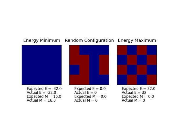
The script ILcheck.py was used to compare the values calculated from the energy(self) and magnetisation(self) functions with the expected values for the magnetisation energy and net magnetisation of a 4x4 Ising lattice. The expected values for the magnetisation energy and net magnetisation of each configuration (Figure 2) agree perfectly with the values calculated by the functions. Therefore the energy(self) and magnetisation(self) functions can be used in later calculations.

Figure 2: Plot of the minimum energy (left), random (center) and maximum energy (right) of a 4x4 Ising lattice computed by ILcheck.py. Blue and red squares denote cells occupied by atoms with spins s=+1 and s=-1, respectively.

Importance sampling and the Monte-Carlo method

Calculating the average interaction energy and magnetisation

Task 6

At temperatures above 0 K thermal energy available causes fluctuations in the number of +1 and -1 spins in the lattice, and thus the system no longer has only 2 microstates. For a system with 100 spins, the number of microstates (configurations) available is $W=2^{100}$. Therefore, to find out which configurations contribute to the average interaction energy and average net magnetisation of the lattice at a given temperature several configurations need to be analysed. One approach to obtain the averages is to calculate the interaction energies, net magnetisations and Boltzmann factors of all the possible configurations of the lattice and then use these values to compute the average interaction energy and average net magnetisation. Such an approach, however, becomes more time consuming as the lattice being analysed increases in size. For example, if the average net magnetisation was calculated on a computer that could analyse 10⁹ configurations per second it would take ca. 1.27x10²¹ s, or ca. 4.02x10¹³ years, to complete the calculation. Not all the possible configurations of a lattice will contribute to its average interaction energy and average magnetisation at a given temperature therefore some configurations can be ignored when calculating the averages. This can be achieved using importance sampling and the Monte-Carlo method.

NJ: the temperatures are in reduced units, not Kelvin! Even at T=0, there are still 2^100 microstates — it's the number of accessible microstates which is determined by the temperature.

Task 7

montecarlostep(self, T) and statistics(self) functions in class IsingLattice

def montecarlostep(self, T):
        #this function performs a single Monte Carlo step
        a0, energy, magnetisation= self.lattice, self.energy(), self.magnetisation()
        #the following two lines will select the coordinates of the random spin for you
        random_i = np.random.choice(range(1, self.n_rows))
        random_j = np.random.choice(range(1, self.n_cols))
        #the following line flips one spin at [random_i, random_j] in the lattice
        self.lattice[random_i, random_j]=-self.lattice[random_i, random_j]
        a1, E1, M1= self.lattice, self.energy(), self.magnetisation()
        dE=E1-energy #E1= energy of random configuration
        #the following line will choose a random number in the range [0,1)
        random_number = np.random.random()
        if dE<=0: 
            a0, energy, magnetisation= a1, E1, M1 #random configuration is accepted
        elif dE>0:
            if np.exp(-dE/T)>=random_number:
                a0, energy, magnetisation= a1, E1, M1 #random configuration is accepted
            elif np.exp(-dE/T)<random_number:
            #The line below changes self.lattice back to a0 if the condition in the elif statement in the line above is met
                self.lattice[random_i, random_j]=-self.lattice[random_i, random_j] #random configuration is rejected
        #the following lines update the running sum of E, E2, M and M2
        self.E=self.E+energy
        self.E2=self.E2+(energy)**2
        self.M=self.M+magnetisation
        self.M2=self.M2+(magnetisation)**2
        self.n_cycles+=1
        # the function should end by calculating and returning both the energy and magnetisation:
        return energy, magnetisation
        
    def statistics(self):
        #this function calculates the values for the averages of E, E*E (E2), M, M*M (M2), and returns them along with 
        #the number of cycles n_cycles
        aveE = self.E/(self.n_cycles)
        aveE2 = self.E2/(self.n_cycles)
        aveM = self.M/(self.n_cycles)
        aveM2 = self.M2/(self.n_cycles)
        return aveE, aveE2, aveM, aveM2, self.n_cycles

NJ: You are only selecting random spins between 1 and the length here, so the first row and column can't be chosen. This was an error in the original version of the script, and I think you must have corrected it later because the rest of the results look good.

Task 8

Figure 3: Simulation of 8x8 lattice with the Monte-Carlo algorithm using ILanim.py. Top: plot of current lattice configuration, middle: plot ofinteraction energy per spin (E/spin) vs number of steps, bottom: plot of net magnetisation per spin (M/spin) vs number of steps

Output of a simulation with ILanim.py

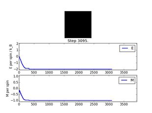
A simulation of an 8x8 lattice at 0.5 K for 3122 steps was run using ILanim.py to yield the plots in Figure 3. The plots of the interaction energy per spin (E/spin) vs number of steps and net magnetisation per spin (M/spin) vs number of steps show that, at 0.5 K, the lattice reaches its equilibrium state after around 400 steps of the simulation. After this equilibration period, no significant fluctuations in E/spin and M/spin are observed, and both E/spin and M/spin remain roughly constant. The averages <E/spin>=-1.9321748878923768 and <M/spin>=-0.9740150544522742 obtained at the end of the simulation period are almost in perfect agreement with the expected values for the interaction energy per spin and the magnetisation per spin for an 8x8 lattice at 0 K, which are E/spin=-128/64=-2 and M/spin=-64/64=-1. Below the Curie temperature T_C of a ferromagnetic material it is expected that spontaneous magnetisation in the material will occur and that the average magnetisation $⟨M⟩\ne 0$. The plot of M/spin vs number of steps, however, shows that the magnetisation in the lattice is initially closer to 0 than expected; this is because the code generates the starting configuration at random, and this configuration is very likely higher in energy than the lowest energy configuration.

Output of ILanim.py from statistics(self) function

('Cycles elapsed = ', 3122)
Averaged quantities:
('E = ', -1.9321748878923768)
('E*E = ', 3.810370455637412)
('M = ', -0.9740150544522742)
('M*M = ', 0.9618102128042921)

Accelerating the code

Task 9 NB: In this task ILtimetrial.py was run on a computer with a HP intel CORE i7 vPro processor The energy(self) and magnetisation(self) functions were tested using ILtimetrial.py which measured the time taken to run the montecarlostep(self, T) function 2000 times. The average time taken to perform 2000 Monte-Carlo steps $⟨t⟩$ was calculated from times obtained $t_i$ from 1000 repeat runs of ILtimetrial.py and the standard error in this average $dt$ was calculated using:

$$\begin{gathered} dt=\frac{1}{N}\sqrt{\sum _i^N \\ (t_i-⟨t⟩ \\ {)}^2}=\frac{\sigma }{\sqrt{N}} \end{gathered}$$

where the number of repeats $N=1000$ and $\sigma$ is the standard deviation. For the original energy(self) and magnetisation(self) functions the average time in seconds $$\begin{gathered} ⟨t⟩ \\ =4.03727837495\pm 0.0875591890212s \end{gathered}$$.

Task 10

The energy(self) and magnetisation(self) functions were rewritten using NumPy functions to optimise them for speed.

Optimised function to calculate magnetisation energy IsingLattice

def energy(self):
    #this function calculates the interaction energy
    energy=-(np.sum(np.multiply(self.lattice, np.roll(self.lattice, 1, axis=0)))+np.sum(np.multiply(self.lattice, np.roll(self.lattice, 1, axis=1))))
    return energy

Optimised function to calculate net magnetisation in IsingLattice

def magnetisation(self):
    #this function calculates the net magnetisation
    return np.sum(self.lattice)

Task 11

The optimised energy(self) and magnetisation(self) functions were tested using ILtimetrial.py and the average time taken to perform 2000 Monte-Carlo steps $⟨t⟩$ was calculated from times obtained $t_i$ from 1000 repeat runs of ILtimetrial.py. This average time was calculated to be $$\begin{gathered} ⟨t⟩ \\ =0.2235433141795\pm 0.00246861627917s \end{gathered}$$ which is significantly faster than the average time observed for the original energy(self) and magnetisation(self) functions.

NJ: Good. Are you surprised by how much of a difference this makes?

The effect of temperature

Task 12

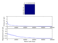
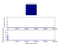
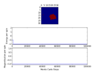
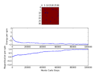
The plots of E/spin vs number of steps and M/spin vs number of steps in Figure 3 show that there is a period in the simulation before the lattice reaches its equilibrium state. The montecarlostep(self, T) function in its current form calculates the running sums of the attributes self.E, self.E2, self.M and self.M2 from the start of the simulation. In order to obtain more accurate averages, corrections to the montecarlostep(self, T) and statistics(self) functions are required so that during the calculation of the averages aveE, aveE2, aveM and aveM2 the energy and magnetisation values from the equilibration period are ignored. Before any corrections to the montecarlostep(self, T) and statistics(self) functions can be made the number of equilibration steps during which the running sum is not calculated must be determined. The script ILfinalframe.py was used to run simulations of 2x2, 8x8 and 32x32 lattices at 0.25 K, 0.5 K, 1 K and 1.75 K. This temperature range was chosen so that all simulations were run below the observed critical temperatures of 2-dimensional Ising lattices (ca. 2-2.5 K). The plots thus obtained are shown below:

Plots from ILfinalframe.py

T (K, horizontal) vs runs (vertical)	2x2	8x8	32x32
0.25
0.5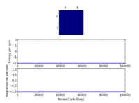
1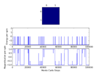
1.75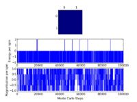

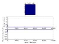
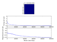
Plots of energy per spin vs Monte-Carlo steps and magnetisation per spin vs Monte-Carlo steps from simulations at 0.25 K and 0.5 K show that no noticeable equilibration period is observed for the 2x2 lattice system and only a very short equilibration period of ca. 1000 steps is observed for the 8x8 lattice whereas the 32x32 lattice system exhibits a much longer equilibration period of ca. 70000-80000 steps. At 0.25 K and 0.5 K, the lattice systems are close to absolute zero so the equilibrium states of each lattice are expected to have average energy per spin of approximately $E=-DJ=-2$ and average magnetisation per spin of approximately $M=-1$ or $M=1$, depending on the initial configuration. The energy per spin vs Monte-Carlo steps and magnetisation per spin vs Monte-Carlo steps curves both converge to the expected energy per spin and magnetisation per spin values at 0.25 K and 0.5 K for all of the lattices simulated therefore showing that the lattices were able to reach the equilibrium state. Plots of energy per spin vs Monte-Carlo steps and magnetisation per spin vs Monte-Carlo steps from simulations at 1.0 K and 1.75 K show that only the 8x8 and 32x32 lattices were able to reach an equilibrium state and for both lattices the length of the equilibration periods were similar to those at 0.25 K and 0.5 K, however the 2x2 lattice exhibits large, rapid fluctuations in its energy per spin and magnetisation suggesting its Curie temperature has been reached and the 2x2 lattice system is undergoing a phase transition. At all temperatures at which the simulation was performed, the 32x32 lattice system exhibited a steep drop in its energy per spin and magnetisation per spin only within the first 40000-50000 steps of the simulation, which is far longer than the typical equilibration periods of the 8x8 lattice within the temperature range of the simulations. Therefore, it is reasonable to ignore the first 40000 steps of the simulation when calculating the averages of self.E, self.E2, self.M and self.M2.

Corrected montecarlostep(self, T) and statistic(self) functions in class IsingLattice

    def montecarlostep(self, T):
        # complete this function so that it performs a single Monte Carlo step
        a0, energy, magnetisation= self.lattice, self.energy(), self.magnetisation()
        #the following two lines will select the coordinates of the random spin for you
        random_i = np.random.choice(range(0, self.n_rows))
        random_j = np.random.choice(range(0, self.n_cols))
        self.lattice[random_i, random_j]=-self.lattice[random_i, random_j]
        a1, E1, M1= self.lattice, self.energy(), self.magnetisation()
        dE=E1-energy
        #the following line will choose a random number in the range [0,1) for you
        random_number = np.random.random()
        if dE<=0:
            a0, energy, magnetisation= a1, E1, M1
        elif dE>0:
            if np.exp(-dE/T)>=random_number:
                a0, energy, magnetisation= a1, E1, M1
            elif np.exp(-dE/T)<random_number:
                self.lattice[random_i, random_j]=-self.lattice[random_i, random_j]
        #the following lines determine the step after which the running sum is performed
        if self.n_cycles<40000:
            self.n_cycles+=1 #increases n_cycles until it reaches end of equilibration period (40000 steps)
        elif self.n_cycles>=40000:
            self.E=self.E+energy
            self.E2+=(energy)**2
            self.M+=magnetisation
            self.M2+=(magnetisation)**2
            self.n_cycles+=1
        # the function should end by calculating and returning both the energy and magnetisation:
        return energy, magnetisation
        
    def statistics(self):
        # complete this function so that it calculates the correct values for the averages of E, E*E (E2), M, M*M (M2), and returns them
        #along with the number of cycles
        #self.n_cycles is subtracted by 40000 as the running sums of E, E2, M and M2 are not performed until the 40000th step
        aveE=self.E/(self.n_cycles-40000)
        aveE2=self.E2/(self.n_cycles-40000)
        aveM=self.M/(self.n_cycles-40000)
        aveM2=self.M2/(self.n_cycles-40000)
        return (aveE, aveE2, aveM, aveM2, (self.n_cycles-40000))

Task 13 From the plots in task 12 it was observed that large lattice systems, such as a 32x32 lattice only reached an equilibrium state after around 80000 steps and it was determined that the first 40000 steps of the simulation would be ignored when calculating the averages of self.E, self.E2, self.M and self.M2. Therefore, simulations in later calculations will be performed with 140000 steps. The plot in Figure 4 was obtained with ILtemperaturerange.py which performed a 140000 step simulation of an 8x8 lattice in the temperature range 0.25 K - 5 K, plotting the average energy/spin and average magnetisation/spin at 0.1 K intervals.

Figure 4: Plot of average energy/spin vs temperature and average magnetisation/spin vs temperature of an 8x8 lattice.

The plot shows that the 8x8 lattice undergoes a phase transition in the region of 2 K - 3 K as there are large fluctuations in the magnetisation/spin which drops from ca. 1 to ca. 0 within the 2 K - 3 K, and the energy/spin increases from ca. -2 to ca. 0 in this region. The size of the error bars for the magnetisation/spin and energy/spin suggests there is only a small spread in the magnetisation/spin and energy/spin values at each temperature.

ILtemperaturerange.py

from IsingLattice import *
from matplotlib import pylab as pl
import numpy as np

n_rows = int(input("number of rows: ")) #prompts user to input the number of rows in the lattice

il = IsingLattice(n_rows, n_rows)
il.lattice = np.ones((n_rows, n_rows))
spins = n_rows**2
runtime = 140000
times = range(runtime)
temps = np.arange(0.25, 5.0, 0.1)
energies = []
magnetisations = []
energysq = []
magnetisationsq = []
#the errE and errM lists store the standard errors in the energy/spin and magnetisation/spin at each temperature, respectively
errE=[]
errM=[]
for t in temps:
    for i in times:
        if i % 100 == 0:
            print(t, i)
        energy, magnetisation = il.montecarlostep(t)
    aveE, aveE2, aveM, aveM2, n_cycles = il.statistics()
    energies.append(aveE)
    energysq.append(aveE2)
    magnetisations.append(aveM)
    magnetisationsq.append(aveM2)
    #The following 2 lines calculates the standard error in the average energy and average magnetisation
    errE.append(((aveE2-(aveE**2))**0.5)/(spins*(n_cycles)**0.5))
    errM.append(((aveM2-(aveM**2))**0.5)/(spins*(n_cycles)**0.5))
    #reset the IL object for the next cycle
    il.E = 0.0
    il.E2 = 0.0
    il.M = 0.0
    il.M2 = 0.0
    il.n_cycles = 0.0
fig = pl.figure()
enerax = fig.add_subplot(2,1,1)
enerax.set_ylabel("Energy per spin")
enerax.set_xlabel("Temperature")
enerax.set_ylim([-2.1, 2.1])
enerax.plot(temps, np.array(energies)/spins, label=str(n_rows)+"x"+str(n_rows))
enerax.errorbar(temps, np.array(energies)/spins, yerr=np.array(errE), marker="") #plots error bars for each point in E/spin vs T

pl.legend()
magax = fig.add_subplot(2,1,2)
magax.set_ylabel("Magnetisation per spin")
magax.set_xlabel("Temperature")
magax.set_ylim([-1.1, 1.1])
magax.plot(temps, np.array(magnetisations)/spins, label=str(n_rows)+"x"+str(n_rows))
magax.errorbar(temps, np.array(magnetisations)/spins, yerr=np.array(errM), marker="") #plots error bars for each point in E/spin vs T

pl.legend()
pl.show()

final_data = np.column_stack((temps, energies, energysq, magnetisations, magnetisationsq))
np.savetxt(str(n_rows)+"x"+str(n_rows)+".dat", final_data)

The effect of system size

Task 14

Using ILtemperaturerange.py, plots of the average energy/spin vs temperature and average magnetisation/spin vs temperature were generated for lattices of different sizes (2x2, 4x4, 16x16, 32x32) in addition to the plot for the 8x8 lattice. All of the plots (Figure 5-Figure 9) of the average magnetisation/spin vs temperature show a region in which there are large fluctuations in the average magnetisation/spin and over these regions the average magnetisation/spin drops from ca. +1 to ca. 0, indicating a phase transition from the ferromagnetic phase to the paramagnetic phase of the lattice systems. At lower temperatures, the stabilisation energy due exchange interactions between parallel atomic spins is greater than the thermal energy available in the system so spins tend to align whereas at high temperatures the thermal energy available overcomes the stabilisation energy due to exchange effects between parallel atomic spins causing spins to "flip" and become anti-aligned, thus increasing the system entropy. The plots show that the temperature at which the onset of the phase transition occurs increases on changing the lattice size from 2x2 to 32x32. This is due to small lattices having lower stabilisation energies compared to large lattices, since small lattices will have fewer atomic spins and thus fewer exchange interactions between aligned spins than in large lattices; hence, aligned spins in small lattices require less thermal energy to become anti-aligned than in large lattices. For all the lattices simulated the average energy/spin fluctuates over a wider temperature range than the average magnetisation/spin, which changes more abruptly during a phase transition. Furthermore, the energy/spin of the 2x2, 4x4 and 8x8 converge to ca. 0 energy/spin over a smaller temperature range than the energy/spin of the 16x16 and 32x32 lattices. Therefore, for the simulation to properly model long range fluctuations in the lattice during the phase transition the minimum lattice size should be 16x16.

NJ: Actually the 8x8 lattice typically looks very similar to the larger ones — it's easier to see this when all of the curves are plotted on the same axes.

Figure 5: Plot of average energy/spin vs temperature and average magnetisation/spin vs temperature of a 2x2 lattice.

Figure 6: Plot of average energy/spin vs temperature and average magnetisation/spin vs temperature of a 4x4 lattice.

Figure 7: Plot of average energy/spin vs temperature and average magnetisation/spin vs temperature of an 8x8 lattice.

Figure 8: Plot of average energy/spin vs temperature and average magnetisation/spin vs temperature of a 16x16 lattice.

Figure 9: Plot of average energy/spin vs temperature and average magnetisation/spin vs temperature of a 32x32 lattice.

Heat capacity and locating the Curie temperature

Task 15 The plot in Figure 10 was generated by the script ILheatcapacity.py which calculates the heat capacity from average energy $⟨E⟩$ and average squared energy $⟨E^2⟩$ values calculated for each lattice size by the montecarlostep() and statistics() functions in the IsingLattice class. The heat capacity $C$ is expressed in terms of $⟨X⟩$ and $⟨X^2⟩$ in the following equation:

$C=\frac{⟨E^2⟩-{⟨E⟩}^2}{k_B{T}^2}$

where $T$=temperature and the variance, $\mathrm{V}\mathrm{a}\mathrm{r}[E]=⟨E^2⟩-{⟨E⟩}^2$.

ILheatcapacity.py

#this script plots heat capacity/spin vs T for 2x2, 4x4, 8x8, 16x16 and 32x32 lattices
from IsingLattice import *
from matplotlib import pylab as pl
from numpy import *
import numpy as np
n_rows = 2
fig = pl.figure()
labels, plot_data = [], []
while n_rows <= 32:
    data = np.loadtxt(str(n_rows)+"x"+str(n_rows)+".dat") #loads data from .dat file as an array
    heat_capacity = np.subtract(data[: , 2], data[ : , 1]**2)/((n_rows*data[ : , 0])**2) #calculates heat capacity, here np.subtract(data[: , 2], data[ : , 1]**2) is the variance


    plot_data.append(data[ : , 0]) #appends temperatures in range [0.25, 5] K to plot_data
    plot_data.append(heat_capacity) #appends heat capacities calculated in heat_capacity variable
    labels.append(str(n_rows)+"x"+str(n_rows)+"lattice") #appends labels generated for each lattice size
    n_rows=2*n_rows   
fig = pl.figure()
hcax = fig.add_subplot(2,1,1)
hcax.set_ylabel("Heat capacity/ spin")
hcax.set_xlabel("Temperature (K)")
hcax.plot(plot_data[0], np.array(plot_data[1]), "r", label=str(labels[0])) #plots heat capacity/spin vs T for 2x2 lattice
hcax.plot(plot_data[2], np.array(plot_data[3]), "g", label=str(labels[1])) #plots heat capacity/spin vs T for 4x4 lattice
hcax.plot(plot_data[4], np.array(plot_data[5]), "b", label=str(labels[2])) #plots heat capacity/spin vs T for 8x8 lattice
hcax.plot(plot_data[6], np.array(plot_data[7]), "k", label=str(labels[3])) #plots heat capacity/spin vs T for 16x16 lattice
hcax.plot(plot_data[8], np.array(plot_data[9]), "m", label=str(labels[4])) #plots heat capacity/spin vs T for 32x32 lattice
hcax.legend(loc=2,prop={'size':6})
pl.show()

Figure 10: Plots of heat capacity/ spin vs temperature for 2x2, 4x4, 8x8, 16x16 and 32x32 lattices.

Task 16

IL2heatcapacity.py

#this script plots data from simulations in Python and C++ of a 2-dimensional square Ising lattice
from IsingLattice import *
from matplotlib import pylab as pl
import numpy as np
n_rows=int(input("Enter number of rows: ")) #prompts user to input number of rows in lattice
data=np.loadtxt(str(n_rows)+"x"+str(n_rows)+".dat") #loads data generated by ILtemperaturerange.py
data_from_C=np.loadtxt("../ImperialChemYear3CMPExptmaster/C++_data/"+str(n_rows)+"x"+str(n_rows)+".dat") #loads data from C++ simulation
fig = pl.figure()
hcax = fig.add_subplot(2,1,1)
hcax.set_ylabel("Heat capacity/ spin")
hcax.set_xlabel("Temperature")
#plots heat capacity/ spin vs T from data generated by ILtemperaturerange.py
hcax.plot(data[ : ,0], np.subtract(data[ : ,2], data[ : ,1]**2)/((n_rows*data[ : ,0])**2), "b", label = str(n_rows)+"x"+str(n_rows)+" lattice") 
#plots heat capacity/ spin vs T from data generated by C++ simulation
hcax.plot(data_from_C[ : , 0], data_from_C[ : , 5], "k", label = str(n_rows)+"x"+str(n_rows)+" lattice (C++ data)") 
hcax.legend(loc=2,prop={'size':6})
pl.show()

Figure 11: Plots of heat capacity/ spin (Python simulation) vs temperature and heat capacity/ spin (C++ simulation) vs temperature for 2x2 lattice.

Figure 12: Plots of heat capacity/ spin (Python simulation) vs temperature and heat capacity/ spin (C++ simulation) vs temperature for 4x4 lattice.

Figure 13: Plots of heat capacity/ spin (Python simulation) vs temperature and heat capacity/ spin (C++ simulation) vs temperature for 8x8 lattice.

Figure 14: Plots of heat capacity/ spin (Python simulation) vs temperature and heat capacity/ spin (C++ simulation) vs temperature for 16x16 lattice.

Figure 15: Plots of heat capacity/ spin (Python simulation) vs temperature and heat capacity/ spin (C++ simulation) vs temperature for 32x32 lattice.

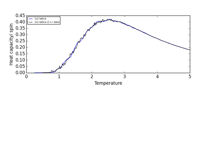
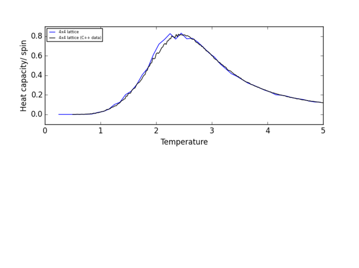
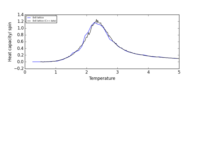
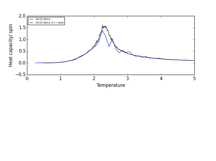
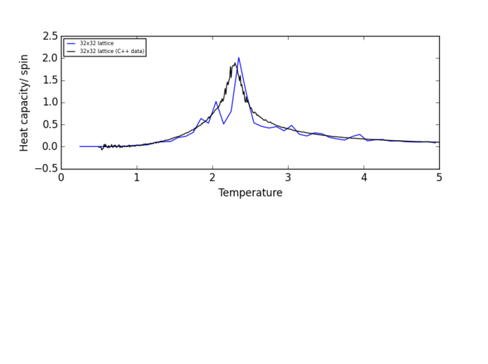
NJ: nice plots

Task 17

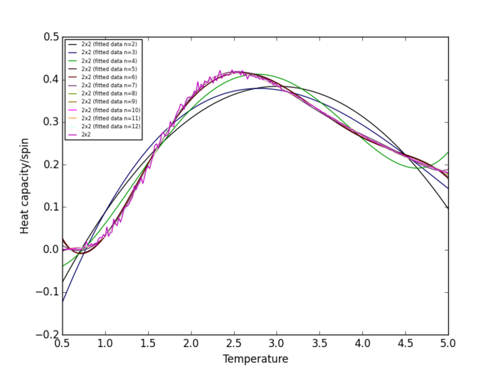
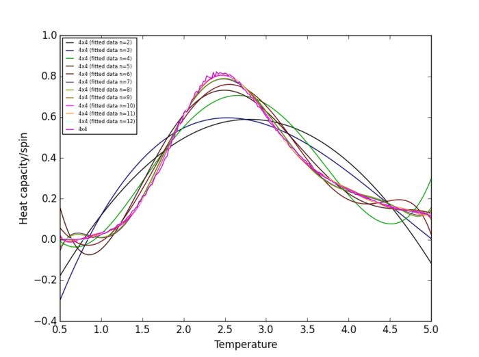
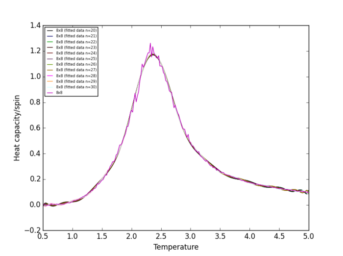
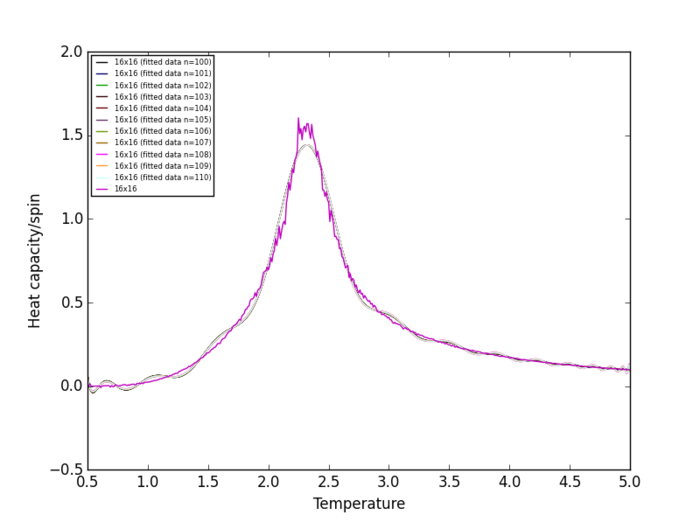
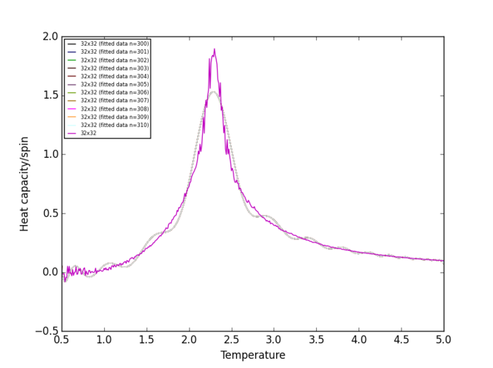
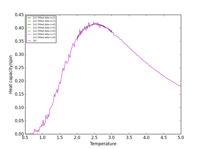
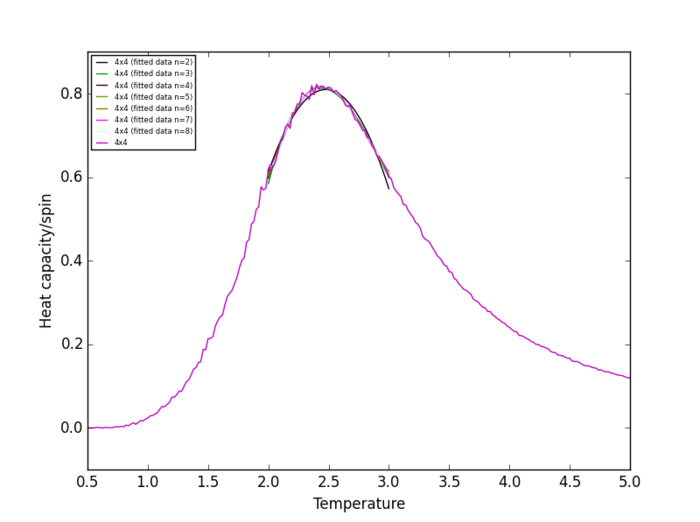
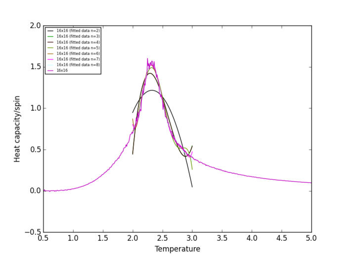
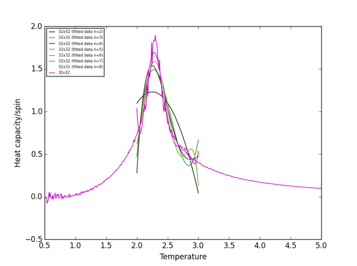
The plots show that the polynomial degree required to obtain a good fit to the heat capacity/spin vs temperature curve increases with increasing lattice size. np.polyfit() issues the following RankWarning when the polynomial degree is above 8, indicating that the solution is "ill conditioned":

C:\Users\rm1412\AppData\Local\Continuum\Anaconda\lib\site-packages\numpy\lib\polynomial.py:588: RankWarning: Polyfit may be poorly conditioned
  warnings.warn(msg, RankWarning)

Therefore, in later parts of this experiment, curves will only be fitted to polynomials with degrees in the range 2-8.

NJ: It's good that you're being careful about this. In general, this is only a warning — as long as you have enough data to do the fit (you can't fit an order 50 polynomial to five datapoints, for example), and the fit looks good, you're probably okay.

ILpolyfitheatcapacity.py

from numpy import *
from matplotlib import pylab as pl

import numpy as np
n_rows=int(input("Enter number of rows: ")) #prompts user to input number of rows in lattice
colour=["000000", "000066", "009900", "330000", "660000", "663366", "669900", "996600", "FF00FF", "FF9933", "CCFFFF"]  
data_from_C=np.loadtxt("../ImperialChemYear3CMPExptmaster/C++_data/"+str(n_rows)+"x"+str(n_rows)+".dat")
T=data_from_C[:, 0]
C=data_from_C[:, 5]    
c=0
fig = pl.figure()
hcax = fig.add_subplot(1,1,1)
hcax.set_ylabel("Heat capacity/spin")
hcax.set_xlabel("Temperature")
lower_limit=int(input("Enter lower limit: ")) #prompts user to enter lowest polynomial degree to fit to heat capacity/ spin vs T data 
deg_list=range(lower_limit,(lower_limit+11)) #generates list of 11 polynomial degree values, starting from lower_limit
for deg in deg_list:
    fit = np.polyfit(T, C, deg)#fits polynomial of degree=deg to heat capacity/ spin vs T from data generated by C++ simulation
    T_min = np.min(T)
    T_max = np.max(T)
    T_range = np.linspace(T_min, T_max, 1000) 
    fitted_C_values = np.polyval(fit, T_range)
    hcax.plot(T_range, fitted_C_values, "#"+colour[c], label=str(n_rows)+"x"+str(n_rows)+" (fitted data n={})".format(deg)) #plots fitted curve
    c+=1
#plots heat capacity/ spin vs T from data generated by C++ simulation
hcax.plot(T, C, color="m", label=str(n_rows)+"x"+str(n_rows))
hcax.legend(loc=2,prop={'size':6})
pl.show()

NJ: nice work with the colours

Figure 16: Plots of heat capacity/ spin (C++ simulation) vs temperature and polynomial curves of different degrees for 2x2 lattice fitted over whole temperature range of simulation.

Figure 17: Plots of heat capacity/ spin (C++ simulation) vs temperature and polynomial curves of different degrees for 4x4 lattice fitted over whole temperature range of simulation.

Figure 18: Plots of heat capacity/ spin (C++ simulation) vs temperature and polynomial curves of different degrees for 8x8 lattice fitted over whole temperature range of simulation.

Figure 19: Plots of heat capacity/ spin (C++ simulation) vs temperature and polynomial curves of different degrees for 16x16 lattice fitted over whole temperature range of simulation.

Figure 20: Plots of heat capacity/ spin (C++ simulation) vs temperature and polynomial curves of different degrees for 32x32 lattice fitted over whole temperature range of simulation.

Task 18

IL2polyfitheatcapacity.py

Plots of heat capacity/spin vs temperature show that the peak in heat capacity/spin occurs in the temperature range 2 K - 3 K for all lattice size. Therefore, the heat capacity/spin vs temperature curves will only be fitted within the range of 2 K to 3 K.

#this function fits a series of polynomial curves to heat capacity data obtained from simulations in C++
from numpy import *
from matplotlib import pylab as pl
import numpy as np
n_rows=int(input("Enter number of rows: ")) #prompts user to input number of rows
min_T = float(input("Enter min_T: ")) #prompts user to input lower limit of temperature range
max_T = float(input("Enter max_T: ")) #prompts user to input upper limit of temperature range
data_from_C=np.loadtxt("../ImperialChemYear3CMPExptmaster/C++_data/"+str(n_rows)+"x"+str(n_rows)+".dat")
T=data_from_C[:, 0]
C=data_from_C[:, 5]
colour=["000000", "009900", "330000",  "669900", "996600", "FF00FF",  "CCFFFF"] #list of various colours of plot lines in hexadecimal code
c=0 #indexes hexidecimal colour codes in colour within the for loop
fig = pl.figure()
hcax = fig.add_subplot(1,1,1)
hcax.set_ylabel("Heat capacity/spin")
hcax.set_xlabel("Temperature")
lower_limit=int(input("Enter lower limit: ")) #prompts user to input smallest polynomial degree
deg_list=range(lower_limit,(lower_limit+7)) #generates list of 6 polynomial degrees starting from lower_limit
#the following lines fit the C_++ simulation data to each polynomial degree in deg_list and then plots the fitted curves and original data
for deg in deg_list:
    selection = np.logical_and(T > min_T, T < max_T)
    peak_T_values = T[selection]
    peak_C_values = C[selection]
    fit = np.polyfit(peak_T_values, peak_C_values, deg)
    T_range = np.linspace(min_T, max_T, 1000) 
    fitted_C_values = np.polyval(fit, T_range)
    hcax.plot(T_range, fitted_C_values, "#"+colour[c], label=str(n_rows)+"x"+str(n_rows)+" (fitted data n={})".format(deg))
    c+=1
hcax.plot(T, C, color="m", label=str(n_rows)+"x"+str(n_rows))
hcax.legend(loc=2,prop={'size':6})
pl.show()

Figure 21: Plots of heat capacity/ spin (C++ simulation) vs temperature and polynomial curves of degrees 2-8 for 2x2 lattice fitted in the region of 2 K - 3 K.

Figure 22: Plots of heat capacity/ spin (C++ simulation) vs temperature and polynomial curves of degrees 2-8 for 4x4 lattice fitted in the region of 2 K - 3 K.

Figure 23: Plots of heat capacity/ spin (C++ simulation) vs temperature and polynomial curves of degrees 2-8 for 8x8 lattice fitted in the region of 2 K - 3 K.

Figure 24: Plots of heat capacity/ spin (C++ simulation) vs temperature and polynomial curves of degrees 2-8 for 16x16 lattice fitted in the region of 2 K - 3 K.

Figure 25: Plots of heat capacity/ spin (C++ simulation) vs temperature and polynomial curves of degrees 2-8 for 32x32 lattice fitted in the region of 2 K - 3 K.

Task 19

ILTcextract.py

#This function fits a polynomial of degree 8 to C++ simulation heat capacity/spin data, then finds the Curie temperature for each lattice size and writes them #along with the lattice side lengths to a file to be read by ILCurieplot.py
from numpy import *
from matplotlib import pylab as pl
import numpy as np
n_rows=2
list_n_rows=[] #this list stores the lattice side lengths
min_T = 2 
max_T = 3 
T_max_values = [] #this list stores the values of the Curie temperatures of lattices with different sizes
deg = 8 
while n_rows<=32:
    #the following lines fit a polynomial of degree 8 to C++ simulation heat capacity/spin data in the region 2 K-3 K
    data_from_C = np.loadtxt("../ImperialChemYear3CMPExptmaster/C++_data/"+str(n_rows)+"x"+str(n_rows)+".dat")
    T = data_from_C[:, 0]
    C = data_from_C[:, 5]
    selection = np.logical_and(T > min_T, T < max_T)
    peak_T_values = T[selection]
    peak_C_values = C[selection]
    fit = np.polyfit(peak_T_values, peak_C_values, deg)
    T_range = np.linspace(min_T, max_T, 1000) 
    fitted_C_values = np.polyval(fit, T_range)
    #the following lines find the Curie temperature, which corresponds to the maximum of the heat capacity/spin vs temperature curve
    C_max = np.max(fitted_C_values)
    T_max = T_range[fitted_C_values == C_max]
    list_n_rows.append(n_rows)
    n_rows=2*n_rows
    T_max_values.append(T_max)

'''ILCurieplot.py'''
#This function reads data from the file produced by ILTcextract.py, fits the Curie temperature data to a straight line, then plots the fitted line and the Curie #temperature data vs 1/lattice side length
final_data = np.column_stack((list_n_rows, T_max_values))
np.savetxt("T_c_determination_data_deg_{}.dat".format(deg), final_data)

from IsingLattice import *
from matplotlib import pylab as pl
from numpy import *
import numpy as np
data=np.loadtxt("T_c_determination_data_deg_{}.dat".format(8))
L=data[ : , 0]
T=data[ : , 1]
fit = np.polyfit(1/L, T, 1)
upp_lim=np.max(1/L)
inverse_L_range=np.linspace(0, upp_lim, 1000)
fitted = np.polyval(fit, inverse_L_range)
settings = dict(boxstyle='square', facecolor='white', alpha=0.5)
text_string=("A= {}".format(fit[0]), "T_c= {}".format(fit[1]))
fig = pl.figure()
ax = fig.add_subplot(1,1,1)
ax.set_ylabel("Peak temperature (K)")
ax.set_xlabel("1/L")
ax.plot(1/L, T, "r", linestyle="", marker="o")
ax.text(0.01, 0.95, text_string, transform=ax.transAxes, fontsize=14, verticalalignment='top', bbox=settings)
ax.plot(inverse_L_range, fitted, "b")
pl.show()

Figure 26: Plot of Peak (Curie) Temperatures vs 1/L for different lattice sizes (L=lattice side length)

NJ: I would adjust the limits a little so that the data is clearer

The plot in Figure 26 was generated by ILCurieplot.py and uses the scaling relation for the Curie temperature of a 2-dimensional lattice of side L T_{C, L}:

$T_{C,L}=\frac{A}{L}+T_{C,\mathrm{\infty }}$

where $A$ is a constant (the slope of the plot in Figure 26) and $T_{C,\mathrm{\infty }}$ is the Curie temperature of the infinite (L=$\mathrm{\infty }$) 2-dimensional Ising lattice (the y-intercept of the plot in Figure 26). The theoretical exact Curie temperature of the infinite 2D Ising lattice can be obtained by solving the following equation for $\frac{k_B{T}_c}{J}$ with the method outlined below:

$$\begin{gathered} sinh(\frac{2J}{k_B{T}_{c,\mathrm{\infty }}} \\ )sinh(\frac{2J^{\prime }}{k_B{T}_{c,\mathrm{\infty }}} \\ )=1 \end{gathered}$$

In this experiment it is assumed that$J=J^{\prime }=1$ where $J$=horizontal coupling constant, $J^{\prime }$=vertical coupling constant

Therefore, $$\begin{gathered} sin{h}^2(\frac{2J}{k_B{T}_{c,\mathrm{\infty }}} \\ )=1 \end{gathered}$$ => $$\begin{gathered} sin{h}^2(\frac{2J}{k_B{T}_{c,\mathrm{\infty }}} \\ )-1=0 \end{gathered}$$

$$\begin{gathered} (sinh(\frac{2J}{k_B{T}_{c,\mathrm{\infty }}} \\ )-1)(sinh(\frac{2J}{k_B{T}_{c,\mathrm{\infty }}} \\ )+1)=0 \end{gathered}$$

Solving $$\begin{gathered} (sinh(\frac{2J}{k_B{T}_{c,\mathrm{\infty }}} \\ )-1)=0 \end{gathered}$$ gives:

$$\begin{gathered} \frac{2}{arcsinh(\frac{2J}{k_B{T}_{c,\mathrm{\infty }}} \\ )}=\frac{k_B{T}_{c,\mathrm{\infty }}}{J}=2.269 \end{gathered}$$

The theoretical exact value thus obtained is noticeably lower than the value obtained from the y- intercept of the plot ($\frac{k_B{T}_{c,\mathrm{\infty }}}{J}=2.29(3d.p.)$) in Figure 26 but both values are still in reasonably good agreement. One major source of error comes from the fitting procedure. Ideally, the heat capacity/spin vs temperature curves obtained from simulations would be fitted over the whole temperature range of the simulation, however, the polynomial degree that can be used to fit the simulation curves is limited by the capabilities of the no.polyfit() function and hence the curves must be fitted within a temperature range in the vicinity of the peak heat capacity/spin. This ignores the rest of the heat capacity/spin vs temperature curve so the fitted curve may not accurately describe the true behaviour of each lattice system, which induces an error in the estimate for $\frac{k_B{T}_{c,\mathrm{\infty }}}{J}$.

NJ: It's more that this function probably isn't a polynomial! The best we can do is approximate it to try to find the peak position.

With regards to the Monte-Carlo simulation, a major source of error in the estimate value was that a finite number of equilibration steps was chosen in the Monte-Carlo simulation for all lattice sizes thus some lattices may be insufficiently equilibrated. Insufficient equilibration is normally a result of the algorithm choosing the starting configuration randomly thus the equilibration period for a simulation varies between runs.

NJ: that's true, but if you simulate for long enough you can assume that this isn't a problem (this is called the Ergodic hypothesis, if you're interested)

Another major source of error arises from the random number generation using the random() function in generating the initial configurations and controlling the single spin 'flip' dynamics. If the random number generator is poor, it could lead to configurational bias in the simulation other than that due the Monte-Carlo algorithm. Configurational bias thus could lead to the simulated lattice being non-ergodic, another possible source of error, as the probability of sampling each possible configuration of the lattice would not be uniform. The finite size effect was observed to be strong in the lattice systems being modelled as the Curie temperatures varied noticeably with lattice size and therefore this could be another source of error in the estimate for $\frac{k_B{T}_{c,\mathrm{\infty }}}{J}$. All of these possible sources of error decrease the accuracy of the $⟨E⟩$ and $⟨E^2⟩$ values used to calculate the heat capacity $C_v$.

NJ: That's a good idea — nowadays, random number generators shipped with scientific software are pretty good.

References

- ↑ G. Gallavotti, The Phase Separation Line in the Two-Dimensional Ising Model, Commun. math. Phys., 1972, 27, 103-136
- ↑ C. K. Hu, Historical Review on Analytic, Monte Carlo, and Renormalization Group Approaches to Critical Phenomena of Some Lattice Models, Chinese J. Phys., 2014, 52, 1-67
- ↑ Third year CMP compulsory experiment/Introduction to the Ising model, https://wiki.ch.ic.ac.uk/wiki/index.php?title=Third_year_CMP_compulsory_experiment/Introduction_to_the_Ising_model, 7th February 2015
- ↑ D.A. Ajadi , L.A. Sunmonu , O.A. Aremu , and J.A. Oladunjoye, 2D-Ising model for Simulation of Critical Phenomena of NiOFe2O3 using Monte Carlo Technique, International Journal of Innovation and Applied Studies, 2014, 9, 1336-1344
- ↑ D. J. Griffiths, Introduction to Quantum Mechanics, Pearson Prentice Hall, Massachusetts, 2nd edn., 2004, pp. 207–208
- ↑ L. Onsager, Crystal Statistics. I. A Two-Dimensional Model with an Order-Disorder Transition, Phys. Rev., 1944, 65, 117