Talk:Mod:YJJ14

JC: General comments: All tasks answered and results look good. Try to expand your written answers more though and use the background theory behind the experiment to explain your results.

Molecular Dynamics: Simulation of Liquids

Velocity Verlet Equation

When applying the Velocity Verlet Equation, it is possible to achieve a good estimate of the positions and velocity of simple liquid particles by varying the timesteps. The following graphs (Figures 1-4) are plotted from data with a timestep of 0.1.

Figure 1: Position varying with time.

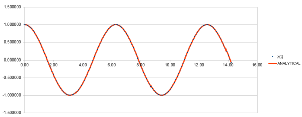
Figure 1 shows that the Velocity-Verlet Equation gives a good estimate of the positions when compared to the analytical positions of a harmonic oscillator $x\left(t\right)=A\cos (\omega t+\varphi )$. The coefficients $A$ and$\mathrm{\Omega }$ are set to 1 and $\varphi$ is set to 0.

Figure 2: Absolute error of between x(t) and analytical positions.

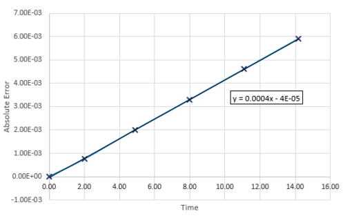
Figure 2 shows the absolute error of positions calculated from the Velocity-Verlet Equation and the positions calculated from a classical harmonic oscillator. Figure 3 shows a linear plot of the maximum absolute errors against time. It can be seen that the error is slowly increasing and should a longer period of time pass, the simulated system will less accurate.

Figure 3: Plot of Maximum Absolute Error in position showing a linear trend.

Figure 4: Total Energy from Velocity-Verlet Algorithm varying with time.

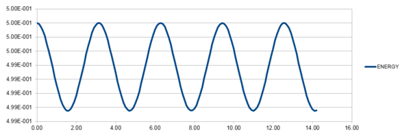
Here the total energy,

$E_{total}=E_p+E_k$

, is calculated using:

$E_p=\frac{1}{2}k{x}^2$

and

$E_k=\frac{1}{2}m{v}^2$

Where $k$ and $m$ are given as 1. The values $x$ and $v$ are estimated with the Velocity-Verlet Equation. It is important that the fluctuation in error calculated here is small, as the total energy of a real system should not change.

---

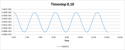
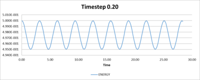
To determine the timestep that is required for the total energy to have less than 1% of fluctuation, trial and error showed that the timestep to achieve small fluctuations in energy in the simulation is 0.2.
This number is large enough so an acceptable amount of time can be run in the simulation, and is small enough so the total energy does not drastically change. It is important that the system simulated is has little change in total energy so the other properties that are measured have a physical significance.

Table 1, shown below, gives a range of timesteps and their associated percentage change in total energy. While Figures 5 to 8 show plots of the fluctuations of total energies for the selected timesteps.

Table 1 - Percentage Changes in Total Energy

Timestep	Percentage %
0.05	0.06
0.10	0.25
0.20	1.00
0.25	1.57

Figure 5: Graph showing the fluctuation in total energy with a timestep of 0.05	Figure 6: Graph showing the fluctuation in total energy with a timestep of 0.10
Figure 7: Graph showing the fluctuation in total energy with a timestep of 0.20	Figure 8: Graph showing the fluctuation in total energy with a timestep of 0.25

JC: Why does the error oscillate? Good choice of timestep.

Lennard-Jones Potential

Separation where potential energy is zero

The separation, $r_0$, for a single LJ interaction where the potential energy is zero is:

$\varphi \left(r\right)=4ϵ(\frac{{\sigma }^{12}}{r^{12}}-\frac{{\sigma }^6}{r^6})=0$

$\therefore$ $(\frac{{\sigma }^{12}}{r^{12}}-\frac{{\sigma }^6}{r^6})=0$

$\therefore$ $\frac{{\sigma }^{12}}{r^{12}}=\frac{{\sigma }^6}{r^6}$

$\therefore$ $\frac{{\sigma }^6}{r^6}=1$

${\mathbf{r}}_{\mathbf{0}}\mathbf{=}\mathit{\sigma }$

Force when potential energy is zero

The force, ${\mathbf{F}}_i$, at the separation $r_0=\sigma$ is given by:

${\mathbf{F}}_i=-\frac{\mathrm{d}U\left({\mathbf{r}}^N\right)}{\mathrm{d}{\mathbf{r}}_i}$

where

$U\left({\mathbf{r}}^N\right)=\sum _i^N\sum _{i\ne j}^N\left\{4ϵ(\frac{{\sigma }^{12}}{r_{ij}^{12}}-\frac{{\sigma }^6}{r_{ij}^6})\right\}$

Substitute,

${\mathbf{F}}_i=-\frac{\mathrm{d}\sum _i^N\sum _{i\ne j}^N\left\{4ϵ(\frac{{\sigma }^{12}}{r_{ij}^{12}}-\frac{{\sigma }^6}{r_{ij}^6})\right\}}{\mathrm{d}{\mathbf{r}}_{\mathrm{i}}}$

Differenciate wrt $r_i$

${\mathbf{F}}_i=-\sum _i^N\sum _{i\ne j}^N\left\{4ϵ(-\frac{12{\sigma }^{12}}{r_{ij}^{13}}+\frac{6{\sigma }^6}{r_{ij}^7})\right\}$

${\mathbf{F}}_i=\sum _i^N\sum _{i\ne j}^N\left\{24ϵ(\frac{2{\sigma }^{12}}{r_{ij}^{13}}-\frac{{\sigma }^6}{r_{ij}^7})\right\}$

Because $r_{ij}=\sigma$ when $U\left({\mathbf{r}}^N\right)=0$

${\mathbf{F}}_i=\frac{24ϵ}{\sigma }$

Equilibrium Separation and well depth

Equilibrium Separation occurs when:

${\mathbf{F}}_i=-\frac{\mathrm{d}U\left({\mathbf{r}}^N\right)}{\mathrm{d}{\mathbf{r}}_i}=24ϵ(\frac{2{\sigma }^{12}}{r^{13}}-\frac{{\sigma }^6}{r^7})=0$

$\therefore (\frac{2{\sigma }^{12}}{r^{13}}-\frac{{\sigma }^6}{r^7})=0$

$\therefore \frac{2{\sigma }^{12}}{r^{13}}=\frac{{\sigma }^6}{r^7}$

And has a value of:

$r_{eq}=\sqrt[6]{2{\sigma }^6}$

With the equilibrium distance, the well depth is found by substituting $r_{eq}$ into $\varphi \left(r\right)$:

$\varphi \left(r_{eq}\right)=-ϵ$

JC: Correct.

Evaluating Integrals

$\int \varphi \left(r\right)\mathrm{d}r=\int 4ϵ(\frac{{\sigma }^{12}}{r^{12}}-\frac{{\sigma }^6}{r^6})\mathrm{d}r$

$=4ϵ(\frac{{\sigma }^{12}}{-11r^{11}}-\frac{{\sigma }^6}{-5r^5})+C$

When $\sigma =ϵ=1.0$:

$\underset{2\sigma }{\overset{\mathrm{\infty }}{\int }}\varphi \left(r\right)\mathrm{d}r\approx -2.48\times 10^{-2}$

$\underset{2.5\sigma }{\overset{\mathrm{\infty }}{\int }}\varphi \left(r\right)\mathrm{d}r\approx -8.18\times 10^{-3}$

$\underset{3\sigma }{\overset{\mathrm{\infty }}{\int }}\varphi \left(r\right)\mathrm{d}r\approx -3.29\times 10^{-3}$

JC: Correct.

Periodic Boundary Conditions

Realistic volumes of liquid cannot be simulated, as they involve many more particles than the usual simulated range of 1000 to 10000 particles.

An example is to show the number of water molecules in 1 mL of water under standard conditions.

$$\begin{gathered} 1 \\ \mathrm{m}\mathrm{L}=1 \\ \mathrm{g} \end{gathered}$$

Number of moles in 1 mL of water: $$\begin{gathered} \frac{1 \\ \mathrm{g}}{18 \\ \mathrm{g} \\ \mathrm{m}\mathrm{o}{\mathrm{l}}^{\mathrm{-}\mathrm{1}}}=5.56\times 10^{-2} \\ \mathrm{m}\mathrm{o}\mathrm{l} \end{gathered}$$

Esimated number of molecules in 1 mL of water: $$\begin{gathered} 5.56\times 10^{-2} \\ \mathrm{m}\mathrm{o}\mathrm{l}\times 6.022\times 10^{23} \\ \mathrm{m}\mathrm{o}{\mathrm{l}}^{\mathrm{-}\mathrm{1}} \end{gathered}$$ $$\begin{gathered} = \\ 3.35\times 10^{22} \end{gathered}$$

In comparison, the estimated volume of 10000 water molecules under standard conditions.

Estimated volume for 10000 water molecules: $$\begin{gathered} \frac{10000}{6.022\times 10^{23}}\times 18=2.99\times 10^{-19} \\ \mathrm{m}\mathrm{L} \end{gathered}$$

Because the volume of simulated water is so drastically different, periodic boundary conditions are applied to better approximate a bulk liquid. This is done by pretending the simulation box is repeated infinitely in all directions, so none of the atoms in the box at the edges are exposed to a vacuum.

In a cubic box that runs from $(0,0,0)$ to $(1,1,1)$. An atom at position $(0.5,0.5,0.5)$ runs along the vector $(0.7,0.6,0.2)$. within one timestep it ends up at $(0.2,0.1,0.7)$ after applying periodic boundary conditions.

JC: Correct.

Reduced Units

It is typical when using Lennard-Jones interactions to work in reduced units, so the results are much more manageable. Reduced units are denoted by a star, and they take the following conversion factors:

Distance $r^{*}=\frac{r}{\sigma }$, Energy $E^{*}=\frac{E}{ϵ}$, Temperature $T^{*}=\frac{k_{B}T}{ϵ}$

The Lennard-Jones parameters for argon are $$\begin{gathered} \sigma =0.34 \\ \mathrm{n}\mathrm{m} \end{gathered}$$ and $$\begin{gathered} ϵ \\ / \\ {k}_B=120 \\ \mathrm{K} \end{gathered}$$.

If the LJ cutoff is $r^{*}=3.2$, in real units:
$r=r^{*}\times \sigma =3.2\times 0.34$

$$\begin{gathered} r=1.088 \\ \mathrm{n}\mathrm{m} \end{gathered}$$

The reduced temperature $T^{*}=1.5$ in real units:
$T=T^{*}\times \frac{ϵ}{k_B}=1.5\times 120$

$$\begin{gathered} T=180 \\ \mathrm{K} \end{gathered}$$

The well depth in $$\begin{gathered} {\mathrm{k}\mathrm{J} \\ \mathrm{m}\mathrm{o}\mathrm{l}}^{-1} \end{gathered}$$:
$ϵ=\frac{k_{B}T\times {\mathrm{N}}_{\mathrm{A}}}{T^{*}\times 1000}=\frac{1.38\times 10^{-23}\times 180\times 6.022\times 10^{23}}{1.5\times 1000}$

$$\begin{gathered} ϵ=0.998 \\ \mathrm{k}\mathrm{J} \\ \mathrm{m}\mathrm{o}{\mathrm{l}}^{\mathrm{-}\mathrm{1}} \end{gathered}$$

JC: Correct.

Equilibration

Creating the simulation box

When two atoms are given random starting coordinates, there is a probability that they will be generated very close together. This can be problematic as it would cause an infinitely high potential to form. This means that it will be difficult to equilibrate during the timescale of the simulation and so may be unable to provide any useful physical properties.

JC: The high repulsive forces that could be generated make the simulation unstable and can cause it to crash without reducing the timestep.

---

In a simple cubic cell, if the distance between lattice points is 1.07722, the number density can be calculated as follows:

$\text{Number density}=\frac{\text{Lattice points}}{\text{Volume of unit cell}}$

In a simple cubic lattice, there is only 1 lattice point in a unit cell.

$\text{Number denisty}=\frac{1}{1.07722^3}=\frac{1}{1.25}=0.8$

---

For a face-centred lattice with a lattice point density of 1.2, the length of the unit cell is:

$\text{Length of unit cell}=\sqrt[3]{\text{Volume of unit cell}}$

$\text{Volume of unit cell}=\frac{\text{Lattice points}}{\text{Number density}}$

There are 4 lattice points in a face centred cubic cell, therefore:

$$\begin{gathered} \text{Length of unit cell}=\sqrt[3]{\frac{4}{1.2}}=1.49 \\ 3sf \end{gathered}$$

---

With a face-centred cubic lattice, create_atoms command would create 4 times as many atoms in a box than when using a simple cubic lattice.

JC: Correct.

Setting the properties of the atoms

The purpose of the following commands in the input script can be found using the LAMMPS manual.

mass 1 1.0
pair_style lj/cut 3.0
pair_coeff * * 1.0 1.0

mass 1 1.0 

This command means that you are defining the mass of the atoms. With a type 1 and with a mass of 1.0 in reduced units

pair_style lj/cut 3.0

This command means that your are simulating paired interactions using a Lennard-Jones potential and cutting off at a distance of 3.0

pair_coeff * * 1.0 1.0

This command defines some of the other coefficients for the simulation. The asterisks correspond to two atoms of any type. The numbers at the end correspond to thecoefficients $\sigma =ϵ=1.0$

---

As we have specified ${\mathbf{x}}_i\left(0\right)$ and ${\mathbf{v}}_i\left(0\right)$, the integration algorithm that we can use is the Velocity-Verlet Algorithm as it will update the position each timestep and the velocity each half-step.

JC: Correct, why is a cutoff used with this potential?

Running the simulation

Figure 9 shows two different formats of command that should both run 100000 steps during a simulation.

### SPECIFY TIMESTEP ### variable timestep equal 0.001 variable n_steps equal floor(100/${timestep}) timestep ${timestep} ### RUN SIMULATION ### run ${n_steps}	timestep 0.001 run 100000
Figure 9: Two different formats of command that should achieve the same output.

The command on the left can easily change the number of steps that it will take during a simulation for a certain timestep.

For example, this specific command shows that a timestep of 0.001 would run 100000 steps. If the timestep was changed to 0.01, the code would automatically calculate the number of steps to be 10000. Both timesteps will eventually run for a total time of 100. This cannot be achieved for the command on the right.

JC: Using variables makes it easier to change parameters of the simulation as all commands which depend on those parameters are updated automatically.

Checking Equilibrium

Figure 10: Graph of total energy against time, timestep: 0.001	Figure 11: Graph of temperature against time, timestep: 0.001
Figure 12: Graph of pressure against time, timestep: 0.001

The Figures 10, 11 and 12 show that equilibrium is reached very rapidly.

• For Total Energy this takes a time of approx: 0.14
• For Temperature this takes a time of approx: 0.30
• For Pressure this takes a time of approx: 0.40

---

Figure 13 shows a graph of all the total energies for all the simulated timesteps, 0.001, 0.0025, 0.0075, 0.01 and 0.015.

Figure 13: Graph of the total energies for the timesteps: 0.001, 0.0025, 0.0075, 0.01 and 0.015.

From these timesteps, it can be seen that the largest timestep that still gives acceptable results is the timestep of 0.01. The worst results occur from the timestep of 0.015, as the total energy simulated from this timestep increases linearly after a short attempt at equilibrating.

However the best timestep to use for future simulations would probably be 0.0025. This timestep achieves the lowest equilibrated energy along with the timestep 0.001. A timestep of 0.0025 would be better because it can simulate for a longer period of time than 0.001, with the best balance.

JC: Good choice of timestep, the average total energy should not depend on the timestep so 0.0075 and 0.01 are not suitable.

Running Simulations Under Specific Conditions

We can change the ensemble of a simulation to measure other properties of a system. In this section the simulations will be run under NpT (isobaric-isothermal) ensembles.

The parameters used in the simulation are two different pressures of 2.5 and 3.0 and temperatures 1.5, 1.7, 1.9, 2.1 and 2.3. All the simulations are run with a timestep of 0.0025, which was the previously determined timestep that gives the best balance between length of simulation and accuracy in results.

Temperature and Pressure Control

To get the target temperature, each velocity will have to by multiplied by the constant factor, $\gamma$.

$\frac{1}{2}\sum _i{m}_i{v}_i^2=\frac{3}{2}N{k}_{B}T$

Multiply each velocity by $\gamma$:

$\frac{1}{2}\sum _i{m}_i{\gamma }^2{v}_i^2=\frac{3}{2}N{k}_B\mathfrak{𝔗}$

Since $E_K=\frac{3}{2}N{k}_{B}T$, substituting this into the equation gives:

${\gamma }^2\frac{1}{2}\sum _i{m}_i{v}_i^2={\gamma }^2\frac{3}{2}N{k}_{B}T=\frac{3}{2}N{k}_B\mathfrak{𝔗}$

This can be simplified and rearranged to:

${\gamma }^{2}T=\mathfrak{𝔗}$

${\gamma }^2=\frac{\mathfrak{𝔗}}{T}$

Therefore

$\gamma =\pm \sqrt{\frac{\mathfrak{𝔗}}{T}}$

JC: Correct.

Examing the Input Script

### MEASURE SYSTEM STATE ###
thermo_style custom step etotal temp press density
variable dens equal density
variable dens2 equal density*density
variable temp equal temp
variable temp2 equal temp*temp
variable press equal press
variable press2 equal press*press
fix aves all ave/time 100 1000 100000 v_dens v_temp v_press v_dens2 v_temp2 v_press2
run 100000

fix aves all ave/time 100 1000 100000 v_dens v_temp v_press v_dens2 v_temp2 v_press2

The three number 100, 1000 and 100000 are the arguments for Nevery, Nrepeat and Nfreq respectively. They determine what timesteps the input values will be used in the average.

Nevery: Number of timesteps between every input number that will be used in the calculation of an average.

Nrepeat: This number refers determines how many input values are averaged. The input values used are the timesteps Nrepeat before the Nfreq.

Nfreq: The multiples of this value of timestep is when averages are calculated.

Ex: For the values Nevery, Nrepeat and Nfreq as 100, 1000 and 100000...

• When nearing timestep = 100000

• 100, 200, 300, 400... 5400, 5500, 5600 ... 99700, 99800, 99900, 100000
• These numbers are 100 timesteps apart from each other. They are the previous 1000 repeats of this timestep which preceded the timestep 100000 when an average is calculated.

This repeats again from 100100 to 200000 where another average of a different set of 1000 values will be calculated.

---

This then means that in this simulation the values such as temperature will be sampled every 100 timesteps. While for the duration of the 100000 timestep simulation, 1000 measurements will contribute to the average.

Finally the total time that is simulated is: number of steps multiplied by the chosen timestep for the simulation.
$100000\times 0.0025=250$

JC: Good.

Plotting the Equations of State

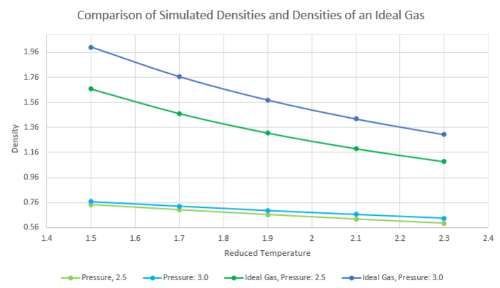
Figure 14 is a plot of density against reduced pressure. As temperature increases, density of the system decreases which in turn suggested that the volume increased when the system increased in energy.

Figure 14: A plot of Density against Reduced Temperature.

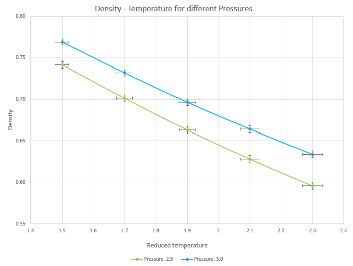
Figure 15 is the same plot with additional lines showing the change in density of ideal gases with different pressures when temperature changes.

The simulated density is lower than the density of an ideal gas, suggesting that in an ideal gas the same number of molecules can occupy less space.

This can be explained as ideal gases assume that there are no interactions between particles. This leads to repulsive forces being non-existent in an ideal gas, allowing particles to be closer to each other.

The simulated systems assume Lennard Jones potentials and when particles become too close to each other, the potential energy increases and they will be pushed apart to occupy a higher volume and lower density.

This discrepancy increases with increased pressure as the difference in densities is larger for the system with a pressure of 3.0 than 2.5.

JC: Why does the discrepancy increase with pressure and decrease with temperature? When is the ideal gas approximation best?

Figure 15: A Density-Temperature Plot with the predicted densities of an ideal gas at the same pressures.

Calculating Heat Capacities Using Statistical Physics

In this section a NVT ensemble was simulated to calculate the heat capacity.

Figure 16 shows a plot of heat capacity at a constant volume over volume. It is showing the variation in energy as temperature changes.

Figure 16: Plot of ^C_v/_V against reduced temperature for two different densities.

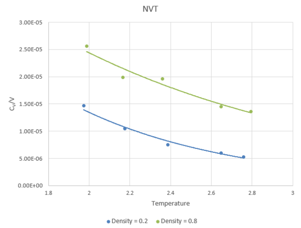
The trend shown is expected. As by increasing the energy of a system by increasing temperature, the systems total capacity for heat decreases. Higher densities allow higher heat capacity/volume because there is a lower volume and hence a higher value of heat capacity.

JC: Can you add a bit more detail to this explanation? Why do you expect the heat capacity to decrease with temperature? The heat capacity is higher at higher densities because there are more particles per unit volume and hence more energy is required to raise the temperature. What function have you used to fit the heat capacity data to and why?

### SET DENSITY OF LATTICE ###
variable density equal 0.2


### DEFINE SIMULATION BOX GEOMETRY ###
lattice sc ${density}
region box block 0 15 0 15 0 15
create_box 1 box
create_atoms 1 box

### DEFINE PHYSICAL PROPERTIES OF ATOMS ###
mass 1 1.0
pair_style lj/cut/opt 3.0
pair_coeff 1 1 1.0 1.0
neighbor 2.0 bin

### SPECIFY THE REQUIRED THERMODYNAMIC STATE ###
variable T equal 2.0
variable timestep equal 0.0025

### ASSIGN ATOMIC VELOCITIES ###
velocity all create ${T} 12345 dist gaussian rot yes mom yes

### SPECIFY ENSEMBLE ###
timestep ${timestep}
fix nve all nve

### THERMODYNAMIC OUTPUT CONTROL ###
thermo_style custom time etotal temp press
thermo 10

### RECORD TRAJECTORY ###
dump traj all custom 1000 output-1 id x y z

### SPECIFY TIMESTEP ###

### RUN SIMULATION TO MELT CRYSTAL ###
run 10000
unfix nve
reset_timestep 0

### BRING SYSTEM TO REQUIRED STATE ###
variable tdamp equal ${timestep}*100
fix nvt all nvt temp ${T} ${T} ${tdamp}
run 10000
unfix nvt
fix nve all nve
reset_timestep 0

### MEASURE SYSTEM STATE ###
thermo_style custom step etotal temp atoms vol
variable energy equal etotal
variable energy2 equal etotal*etotal
variable temp equal temp
variable temp2 equal temp*temp
variable n equal atoms
variable n2 equal atoms*atoms
variable vol equal vol
fix aves all ave/time 100 1000 100000 v_energy v_energy2 v_temp v_temp2
run 100000

variable ave_energy equal f_aves[1]
variable ave_energy2 equal f_aves[2]
variable ave_temp equal f_aves[3]
variable ave_temp2 equal f_aves[4]
variable cv equal ${n2}*(${ave_energy2}-${ave_energy}*${ave_energy})/(${ave_temp}*${ave_temp})
variable cv_v equal ${cv}/${vol}


print “Variables"
print "Temperature: ${ave_temp}"
print "Cv: ${cv}"
print "Cv/V : ${cv_v}"

Structural Properties and the Radial Distribution Function

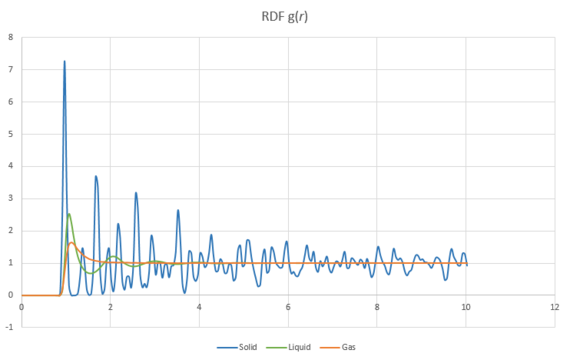
Simulations of Lennard-Jones potentials for the three different phases solid, liquid and a gas were performed. The $g(r)$ and $\int g(r)\mathrm{d}r$ were plotted against distance and are shown in Figure 17 and 18.

Figure 17: RDF of a solid, liquid and gas.

Figure 18: RDF of a solid, liquid and gas.

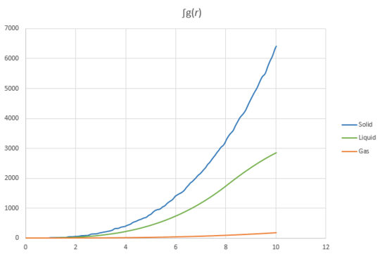The radial distribution function, g(r) shows the probability of finding another atom as a function of distance from a reference atom. In particular the probability of finding a particle on the surface of a sphere as the radius increases.

In all three systems, the RDF initially shows a value of zero before a sharp increase just before r=1. The RDF is zero here because the region is the van der Waals radii of the reference particle. If the probability of finding other particles in this range was larger than 0 then the potential energy of the system would dramatically increase and become very unfavoured because of strong repulsive forces.

In a gas, the probability of finding other particles quickly averages out as the particles in a gas can easily diffuse. So the probability of find more gas particles quickly becomes the same throughout the system. This is very similar to a liquid, though there is a slight increase in organisation of particles immediately surrounding the reference particle.

In solids the RDF shows discrete peaks as you increase the distance from the reference particle. This shows that the structure of a solid is very organised and a particular unit cell of atoms can be repeated periodically in three dimensions of a lattice.

The first three peaks in the RDF for a solid correspond to the first three nearest neighbours in the lattice. This is shown in Figure 19 where some of the nearest neighbour relationships are labelled.

Figure 19: FCC lattice, showing the 1st, 2nd and 3rd nearest neighbours.

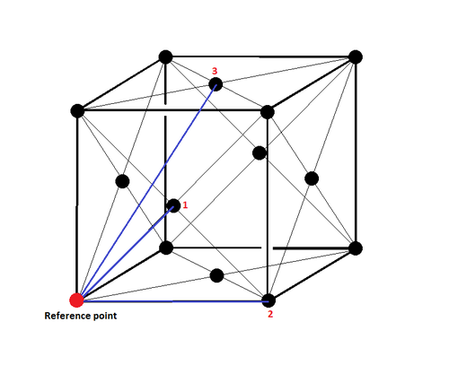
The lattice spacing in the solid system is the distance between the reference atom and the 2nd nearest neighbour.
For a simulation where the density of the system is 1.5 with a temperature of 1.2: the lattice spacing a is 1.375.

The coordination number of the first three peaks are:

• 12 for the first peak and the first nearest neighbour.
• 6 for the second peak and the second nearest neighbour.
• 24 for the third peak and the third nearest neighbour.

JC: The RDF shows that liquids have short ranged order, but solids have long range order. How did you get the coordination numbers for the first 3 peaks? How does the value of the lattice parameter calculated from the RDF compare with the value of the lattice that you set up initially in your simulation? You could have calculated the lattice parameter from the first and third peaks as well using the geometry of the fcc lattice and then taken an average.

Dynamical Properties and the Diffusion Coefficient

Mean Squared Displacement

The mean squared displacement is a measure of the deviation time between the position of a particle and some reference position.

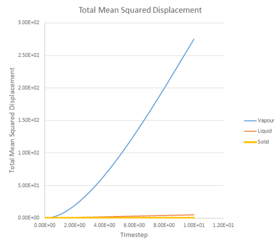
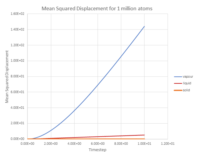
Figure 20 shows a plot of the total mean squared displacement against timestep for the three different phases: a vapour phase, a liquid phase and a solid phase.
It can be seen that displacement occurs significantly faster for the vapour phase than the liquid or solid phases.

Since the mean squared displacement by time, $\frac{\partial ⟨r^2\left(t\right)⟩}{\partial t}$ has already been plotted. The diffusion coefficient can be estimated by extrapolating the linear regions of each line and dividing through by 6 because: $D=\frac{1}{6}\frac{\partial ⟨r^2\left(t\right)⟩}{\partial t}$.

The values of D are shown in Table 2 below. As expected a vapour phase has the largest diffusion coefficient and is significantly large than the diffusion coefficients for liquid and solid phases.

Figure 20: A plot of total mean squared displacement against timestep

Figure 21: A plot of total mean squared displacement against timestep for a simulation of one million atoms.

Table 2 - Values of D for the two simulations of mean squared displacement against time

Phase	D (Area/time) - MSD	D (Area/time) - MSD (million atoms)
Vapour	6.05	3.18
Liquid	8.49 x 10-2	8.72 x 10-2
Solid	7.20 x 10-7	4.39 x 10-6

JC: Plot the MSDs for different phases on different graphs as it is difficult to see the shape of the solid and liquid MSD from your plots. Why is the gas MSD curved initially (ballistic regime) before becoming linear.

Velocity Autocorrelation Function

The Velocity Autocorrelation Function is:
$C\left(\tau \right)=⟨\mathbf{v}\left(t\right)\cdot \mathbf{v}(t+\tau )⟩$

Evaluate the normalised velocity autocorrelation function for a 1D harmonic oscillator.

A 1D harmonic oscillator:

$x\left(t\right)=A\cos (\omega t+\varphi )$

$v(t)=\frac{dx(t)}{dt}=-A\omega \sin (\omega t+\varphi )$

Substitute into the equation for a normalised velocity autocorrelation function: $C\left(\tau \right)=\frac{\underset{-\mathrm{\infty }}{\overset{\mathrm{\infty }}{\int }}v\left(t\right)v(t+\tau )\mathrm{d}t}{\underset{-\mathrm{\infty }}{\overset{\mathrm{\infty }}{\int }}{v}^2\left(t\right)\mathrm{d}t}$

$C\left(\tau \right)=\frac{\underset{-\mathrm{\infty }}{\overset{\mathrm{\infty }}{\int }}(-A\omega \sin (\omega t+\varphi ))\times (-A\omega \sin (\omega (t+\tau )+\varphi ))\mathrm{d}t}{\underset{-\mathrm{\infty }}{\overset{\mathrm{\infty }}{\int }}(-A\omega \sin (\omega t+\varphi ){)}^2\mathrm{d}t}$

$$\begin{gathered} C\left(\tau \right)=\frac{\underset{-\mathrm{\infty }}{\overset{\mathrm{\infty }}{\int }}A\omega \sin (\omega t+\varphi )\times A\omega \sin (\omega t+\omega \tau +\varphi ) \\ \mathrm{d}t}{\underset{-\mathrm{\infty }}{\overset{\mathrm{\infty }}{\int }}{A}^2{\omega }^2{\sin }^2(\omega t+\varphi )\mathrm{d}t} \end{gathered}$$

$$\begin{gathered} C\left(\tau \right)=\frac{A^2{\omega }^2\underset{-\mathrm{\infty }}{\overset{\mathrm{\infty }}{\int }}\sin (\omega t+\varphi )\times \sin (\omega t+\omega \tau +\varphi ) \\ \mathrm{d}t}{A^2{\omega }^2\underset{-\mathrm{\infty }}{\overset{\mathrm{\infty }}{\int }}{\sin }^2(\omega t+\varphi )\mathrm{d}t} \end{gathered}$$

$$\begin{gathered} C\left(\tau \right)=\frac{\underset{-\mathrm{\infty }}{\overset{\mathrm{\infty }}{\int }}\sin (\omega t+\varphi )\times \sin (\omega t+\omega \tau +\varphi ) \\ \mathrm{d}t}{\underset{-\mathrm{\infty }}{\overset{\mathrm{\infty }}{\int }}{\sin }^2(\omega t+\varphi )\mathrm{d}t} \end{gathered}$$

Using double angle formula: $\sin (\alpha \pm \beta )=\sin \alpha \cos \beta \pm \cos \alpha \sin \beta$

$\sin (\omega t+\varphi +\omega \tau )=\sin (\omega t+\varphi )\cos \omega \tau +\cos (\omega t+\varphi )\sin \omega \tau$

$$\begin{gathered} C\left(\tau \right)=\frac{\underset{-\mathrm{\infty }}{\overset{\mathrm{\infty }}{\int }}\sin (\omega t+\varphi )\times [\sin (\omega t+\varphi )\cos \omega \tau +\cos (\omega t+\varphi )\sin \omega \tau ] \\ \mathrm{d}t}{\underset{-\mathrm{\infty }}{\overset{\mathrm{\infty }}{\int }}{\sin }^2(\omega t+\varphi )\mathrm{d}t} \end{gathered}$$

$$\begin{gathered} C\left(\tau \right)=\frac{\underset{-\mathrm{\infty }}{\overset{\mathrm{\infty }}{\int }}{\sin }^2(\omega t+\varphi )\cos \omega \tau +\sin (\omega t+\varphi )\cos (\omega t+\varphi )\sin \omega \tau \\ \mathrm{d}t}{\underset{-\mathrm{\infty }}{\overset{\mathrm{\infty }}{\int }}{\sin }^2(\omega t+\varphi )\mathrm{d}t} \end{gathered}$$

The constants $\cos \omega \tau$ and $\sin \omega \tau$ can be moved to the front.

$$\begin{gathered} C\left(\tau \right)=\frac{\cos \omega \tau \underset{-\mathrm{\infty }}{\overset{\mathrm{\infty }}{\int }}{\sin }^{}(\omega t+\varphi )\mathrm{d}t+\sin \omega \tau \underset{-\mathrm{\infty }}{\overset{\mathrm{\infty }}{\int }}\sin (\omega t+\varphi )\cos (\omega t+\varphi ) \\ \mathrm{d}t}{\underset{-\mathrm{\infty }}{\overset{\mathrm{\infty }}{\int }}{\sin }^2(\omega t+\varphi )\mathrm{d}t} \end{gathered}$$

$$\begin{gathered} C\left(\tau \right)=\frac{\cos \omega \tau \underset{-\mathrm{\infty }}{\overset{\mathrm{\infty }}{\int }}{\sin }^{}(\omega t+\varphi )\mathrm{d}t}{\underset{-\mathrm{\infty }}{\overset{\mathrm{\infty }}{\int }}{\sin }^2(\omega t+\varphi )\mathrm{d}t}+\frac{\sin \omega \tau \underset{-\mathrm{\infty }}{\overset{\mathrm{\infty }}{\int }}\sin (\omega t+\varphi )\cos (\omega t+\varphi ) \\ \mathrm{d}t}{\underset{-\mathrm{\infty }}{\overset{\mathrm{\infty }}{\int }}{\sin }^2(\omega t+\varphi )\mathrm{d}t} \end{gathered}$$

$$\begin{gathered} C\left(\tau \right)=\cos \omega \tau +\frac{\sin \omega \tau \underset{-\mathrm{\infty }}{\overset{\mathrm{\infty }}{\int }}\sin (\omega t+\varphi )\cos (\omega t+\varphi ) \\ \mathrm{d}t}{\underset{-\mathrm{\infty }}{\overset{\mathrm{\infty }}{\int }}{\sin }^2(\omega t+\varphi )\mathrm{d}t} \end{gathered}$$

From here, evaluate the integrals as odd and even functions.

As $sin(x)cos(x)$ is an odd function, and integrating an odd function between equal limits = 0.
The numerator on the right hand side becomes $0$,

$$\begin{gathered} \sin \omega \tau \underset{-\mathrm{\infty }}{\overset{\mathrm{\infty }}{\int }}\sin (\omega t+\varphi )\cos (\omega t+\varphi ) \\ \mathrm{d}t=0 \end{gathered}$$

$\therefore C\left(\tau \right)=\cos \omega \tau +0$

$\therefore C\left(\tau \right)=\cos \omega \tau$

JC: Good, clear derivation.

---

Plotting the VACF for different simulations

Figure 22, shows a plot of the VACF for a liquid and a solid and a harmonic oscillator. If there was no interactions in the system, the atoms would retain their velocities and the plot would show a graph with a horizontal line. However the presence of attractive and repulsive forces between atoms cause them to loose their initial energy and initial velocity.

The minima of the VACFs for the liquid and solid represent the maximum velocities of the atoms when they are travelling in opposite directions to their initial velocities.

The VACF for the liquid has an initial higher velocity because it is at a higher energy system than the solid. However it looses this velocity more rapidly than the solid because of the increased probability in collisions in a more diffusive system. Whereas in the solid, the velocities can much more easily pass back and forth between atoms because how orderly the atoms are arranged in a solid. This leads to a longer period of time where there is a significant oscillation in the velocity of the solid before averaging out like the liquid.

The difference in the VACF for the harmonic oscillator is mainly due to the fact that a harmonic oscillator observes the conservation of energy during an oscillation. This results in a wave where the maxima and minima of the curve have equal amplitudes. In the Lennard Jones liquid and solid, there are atomic interactions that will interfere with this energy conservation and the velocity averages out.

Figure 22: Plot of $cos(\omega \tau )$, and the VACF for a Lennard Jones liquid and a solid.

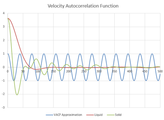
JC: The decorrelation of the VACF is not because of lack of conservation of energy, but is caused by collisions between particles which randomise the velocities of the particles. There are no collisions in the harmonic oscillator.

Estimating D from VACF

As the diffusion coefficient can also be estimated by this equation: $D=\frac{1}{3}\underset{0}{\overset{\mathrm{\infty }}{\int }}\mathrm{d}\tau ⟨\mathbf{v}\left(0\right)\cdot \mathbf{v}\left(\tau \right)⟩$

It can be seen that value is one third of the previously calculated integral for the Velocity Autocorrelation Function.

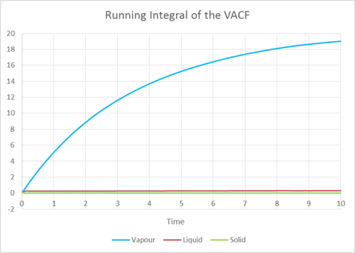
Figures 23-26 are the running integrals of the VACF for the three phases, calculated with the trapezium rule.

Figure 23: Integration of the VACF for a vapour, liquid and solid.	Figure 24: Integration of the VACF for a liquid and solid.
Figure 25: Integration of 1 million atoms of the VACF for a vapour, liquid and solid.	Figure 26: Integration of 1 million atoms of the VACF for a liquid and solid.

The final value of the integral for the vapour, liquid and solid shown in Figures 23-26 divided by three is a good estimate for the diffusion coefficient.

Table 3 shows the diffusion coefficients calculated from the VACF.

Table 3 - Values of D for the two simulations of VACF

Phase	D (Area/time) - VACF	D (Area/time) - VACF (million atoms)
Vapour	6.34	3.27
Liquid	8.49 x 10-2	9.01 x 10-2
Solid	1.14 x 10-5	4.55 x 10-5

If you compare these values of the diffusion coefficients calculated from a VACF to the values of diffusion coefficients calculated from the mean squared displacement, you can see that the values agree with each other rather well. The values of D also are expected, as the diffusion coefficient is largest for the vapour phase and lowest for the solid phase. As diffusion is easiest in a gas and much harder in a rigid solid structure.

The largest error for the estimates of D is probably from the estimation of the integral. The trapezium method tends to overestimate in its calculation of the area under the curve and so the values of the diffusion coefficient using the VACF are larger than the values of D calculated from the MSD.

JC: To calculate the diffusion coefficient from the integral of the VACF we replace the upper limit of the integral by the length of the simulation and this is only valid if the integral has converged by this time, which may be another source of error.