Talk:Mod:Y3 Computational Liquid Simulations
Computational Molecular Dynamics
NOTE: All units used in this experiment are reduced, standardized units unless stated otherwise.
Kinetic and Potential considerations
Errors between classical and velocity-Verlet calculations
| Quantity | Value |
|---|---|
| Spring constant, k | 1.00 |
| Particle mass, m | 1.00 |
| 1.00 | |
| 0.00 | |
| A | 1.00 |
| Timestep | 0.1000 |
A simulation of a simple harmonic oscillator was created and the positions of the particle predicted using both the velocity-Verlet algorithm (1) and the classical solution for such a system (2). Many of the parameters were kept as unit values for simplicity and can be considered as reduced quantities of their actual counterparts.
NJ: Analytical solution is a better way to put it.
(1)
- (2)
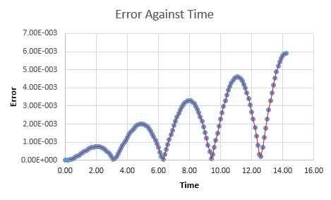
The absolute error between the two values of displacement were then calculated for each timestep by absolute subtraction.
Relationship between the errors and time
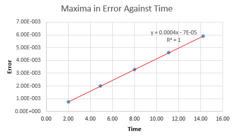
Inspection of a plot of error against time shows several easily visible maxima. The values of error at these points were estimated and these were then plotted against time yet again, to yield a linear positive relationship between the time the simulation runs and the error that the system produces. The equation of the line is calculated to be y = 0.00044x - 7E-5 with an R-squared value of 1. NJ: So the errors accumulate with time?
Optimization of timestep to balance error minimization and simulation utility
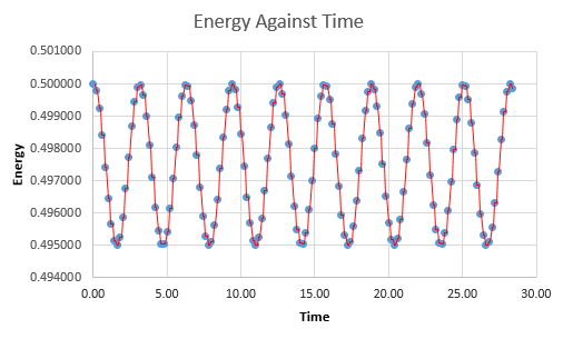
The total energy of the oscillating system should, by right, be constant. However, due to the mathematical, "fitted" nature of the calculations to the scenario, this may not necessarily be the case. A plot of total energy against time of the system (using the velocity-Verlet solutions for kinetic energy, not classical and the equation for potential energy of a spring) gives a non-linear fluctuating line. This plot has a maximum of 0.5, and the minimum value to which it may fall to is dependent on the timestep used in the simulation.
Due to the inherent error in the total energy, it is important to balance the timestep- a value to low will be computationally expensive as it results in an increased sampling rate. A timestep too high, however, also has drawbacks as the low sampling rate may cause inaccuracies in the real time simulation of the system due to "gaps" in the calculations. The timestep was adjusted to 0.2000 as this resulted in a maximum deviation of only 1% (i.e a minimum of 0.495), whilst still being large enough to not be too calculation intensive.
Electrostatic considerations
The significance of σ in the Lennard-Jones
A single Lennard-Jones potential interaction is given by the formula (3):
(3)
By definition, σ is the separation of the two particles at which there no potential energy (the only other place on the Lennard-Jones plot that has this property is where the separation is infinity). This can be proven by setting the potential term, Φ, to 0.
Knowing that ε is constant for this specific interaction,
Forces at zero potential
It is known from classical physics that the negative differential of the potential acting on an object with respect to its position (displacement from the source of the potential) will give the value of force acting on it. Therefore the force acting on a body in a Lennard-Jones interaction is soluble for when the potential energy is zero (r = σ):
therefore at a separation of r = σ:
Equilibrium at the potential well
At equilibrium, the oscillating particle is said to experience no force and so the above equation for force can be equated to zero as well, giving:
rearranging for r in these conditions gives the separation of the system in terms of σ:
Substituting this value into the Lennard-Jones equation, (3), then yields the potential well depth:
(3)
This is also defined in the Lennard-Jones, as ε is representative of the depth of the potential well.
Simple integrations of the Lennard-Jones
Considering a simple Lennard-Jones interaction:
upon applying a simplification where the paramaters σ = ε = 1:
evaluates to the following for different lower limits (2σ, 2.5σ and 3σ):
Behavior of liquid particles in a simulation
A realistic volume of liquid contains too many particles, and is thus too expensive to be simulated with the given computational power. The number of particles considered for calculations will tend to be from 1000 to 10000.
Consider a sample of water at standard conditions with volume 1 cm3- due to the density of water it is known that such a sample will weigh exactly 1 gram. Dividing this by the molar mass of water (18 g mol-1) gives us the number of moles present (0.056 moles) and this value is then multiplied by Avogadro's constant to give the number of molecules present. This works out to be 3.34E22 which is indeed a very intensive amount to have to simulate for such a small volume.
Working in reverse, it is possible to find out what range of volumes can be run with reasonable output time: 10000 molecules is within such a range. Dividing this by the Avogadro's constant gives the number of moles that such a quantity of water makes up (1.66E-20 moles) and this can be multiplied by 18 to yield the mass (and hence volume) of water such a sample size corresponds to. This gives 2.99E-19 cm3.
In order to imitate that the sample is part of a larger, more realistically scaled system, the molecules under consideration are said to be in a box of predetermined volume which is repeated infinitely in all directions. When a particle passes through a boundary on the box, it disappears and reappears on the opposite side of the box (maintaining its velocity at the time of crossing). For example, an atom at position (0.5, 0.5, 0.5) in a box of dimensions (1, 1, 1) with a movement vector (0.7, 0.6, 0.2) will appear at position (0.2, 0.1, 0.7) after a single timestep has passed in the simulation. The end position of any particle can be calculated by adding the x, y and z movement vectors to its current position. If the new position vector has a value which exceeds it's respective axes' dimension of the box, the difference between the two values becomes the new position (e.g considering x: 0.5 + 0.7 = 1.2, 1.2 - 1 = 0.2).
This ensures that the number of molecules in the sampling volume remains constant without inhibiting the movement of actual particles.
Reduced units
For the sake of simplicity and ease of numerical manipulation, reduced units are used in almost all calculations in this experiment. Previously there was no need for any differentiation between symbols of reduced and real values however such a need may come into play soon. Examples of reduced units include:
- Distance
- Energy
- Temperature
For example, consider Argon (σ = 0.34 nm, ε/kB = 120 K). If the Lennard-Jones cutoff is r* = 3.2, its real unit value would be 1.088 nm. The well depth, ε, would be 1.66E-21 kJ mol-1 and the real value of a reduced temperature, T*, of 1.5 would be 180 K. These are solved easily by substituting the appropriate values into the equations above, and greatly simplify operations and understanding of the data until real world values are needed.
NJ: I think your well depth is in Joules, you need to do the conversion to "per-mole"
Computational Simulations
Simulation basics: Particles and samples
The first thing that must be done when simulating the liquid is to arrange the particles being considered in an ordered simple cubic lattice and letting them settle into a more favorable configuration by themselves. This is better than simply assigning each particle a random position in the boundary as such a method can be problematic when, for example, two particles are given the same position, or placed very close together- this would cause them either to superimpose over one another and become one "fused together" particle or their close proximity would invoke a major repulsive force that would disrupt the rest of the system- thus creating an inaccurate measurement of thermodynamic properties for the starting conditions given.
NJ: Fusing together isn't possible, but good otherwise.
The simulation being used for this experiment is known as LAMMPS, and simulations are described and run from starting input files which contain the commands needed to set up the whole system and initialize the starting conditions. Some of the setup lines in the code read:
lattice sc 0.8
Lattice spacing in x,y,z = 1.07722 1.07722 1.07722
This tells the simulation to create a lattice of sides 1.07722 (reduced units) and to place 0.8 lattice points per unit volume into it. This can be confirmed working backwards- finding the number of lattice points per unit volume to find the number density:
This method is also applicable for other types of lattice. Considering a face-centered cubic lattice (which has 3 lattice points per unit cell) of number density 1.2:
NJ: 4 lattice points per cell!
It is calculated that such a cell will have sides 1.36 reduced units.
NJ: Error due to the previous mistakes. Should be ~1.49
Simulation basics: Fundamental LAMMPS Commands
create_atoms
There is a command in LAMMPS known as create_atoms [type] [region] which places an atoms of a certain type (depending on the argument) at each lattice point in a selected region. For example, invoking the create_atoms command on the face-centered cubic lattice earlier will result in the creation of 3 atoms (as an example, if the sides of the lattice is scaled up by a factor of 10 to 13.6, it would make 3000 atoms).
mass
The mass [type] [mass] command defines the mass of a specific atom type. After this quantity has been defined, all atoms of that type will inherit the given properties. So the code mass 1 1.0 will set the mass of atom type 1 to 1.0 reduced units.
pair_style
The pair_style [style] [parameter] command tells the LAMMPS software how to compute its pair interactions. For example, the code being inspected uses pair_style lj/cut 3.0 which tells the simulation software that its pair interactions are of Lennard-Jones type, but to cut off the interactions (i.e Coulomb) at a distance of 3.
NJ: There are no Coulombic interactions, it's the LJ component which is truncated.
pair_coeff
The pair_coeff [type] [type] [factor] [factor] tells LAMMPS of the asymmetry of interactions between two types of atoms. In the code used, the line pair_coeff * * 1.0 1.0 is seen- the asterisk, *, is representative of all the atom types and the two 1.0 parameters mean that the interactions are symmetric. The code says that for this particular simulation, all particles have equal, symmetric interactions with each other with no bias.
NJ: What do you mean by coefficients?
Simulation basics: Methods and technique
As seen before, there is more than one way to calculate the trajectory of a system, whether classically or through integration. For the specific simulation, the initializing code specifies the starting displacement and velocities of the particles and so the most fitting method of calculating the future states of the computed run is the velocity-Verlet algorithm as it uses these quantities directly without much need for manipulation.
A closer look at the code in the starting file reveals that a variable is used to specify values of timestep, rather than simply typing in the values explicitly- this may seem redundant since all instances of timestep are being replaced with the same thing but it has its advantages. The main advantage being that if the timestep ever need to be changed, using the one variable method is more efficient as only one value need be touched for the new one to be carried through all the code. If each value for timestep were to be typed out manually, it would take much longer as one would have to find each time it comes up- and this may lead to errors if all the new numbers do not match up.
NJ: This section makes sure that the time simulated (nsteps*dt) is the same no matter what timestep is chosen.
Finding equilibrium in the systems
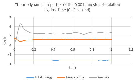
Five simulations were run in LAMMPS- for generic atoms with varying timesteps within the experiment. The log files were loaded into a spreadsheet processing software and plots of thermodynamic data were obtained. For small values of elapsed time, the plots fluctuate as the system reaches equilibrium from its initial ordered lattice state. A stable system is characterized by steady, and relatively constant values which do not fluctuate greatly. It appears that the 0.001 timestep simulation reaches equilibrium approximately 0.3 seconds into the run.
NJ: Not seconds! Reduced time.
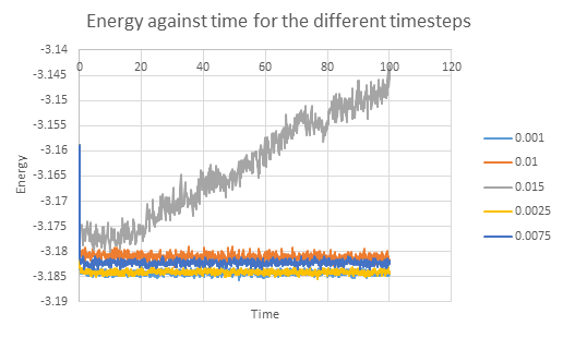
The plots of total energy against time for all the simulations run were then superimposed. It is immediately clear that a timestep of 0.015 is flawed and does not give sensible data. By studying the plots, the optimal timestep can be determined- the 0.001 and 0.0025 runs have the lowest, but almost the same energy which suggests that decreasing the timestep further will only be more computationally expensive whilst not providing a worthwhile increase in accuracy. It makes sense to choose the 0.0025 timestep for simulations as it has the balance between minimization in energy and optimal use of computer resources. Choosing 0.01 as a timestep will also give acceptable results, but with values of a higher deviation from real life.
NJ: Not really - the average energy shouldn't depend on the timestep that you chose.
Technical Interlude
Correction constant, γ
As per the equipartition theorem, all the particles in a system that is in thermal equilibrium will have the same energy of . Multiplying this by three, which is the number of degrees of freedom and multiplying by the number of particles, gives the average kinetic energy of the system:
Equating this to kinetic energy:
(4)
At each timestep, the left hand side of the equation is used to calculate the kinetic energy of the system. This is then divided by to solve for the current temperature of the system at that moment in time. The temperature of the system will tend to fluctuate and will thus deviate from the temperature that the system needs to be if held constant (as specified in the starting input file for NpT ensembles, seen later).
In order to keep the temperature constant, the velocity of the particles needs to be constantly scaled. This is achieved by multiplying each velocity by a constant factor, γ to get the value we need. The equation above can then be rewritten, with the desired temperature :
(5)
The operation can be performed to yield an expression for γ in terms of the current temperature of the system, T, and the desired temperature :
NJ: I'd like to see just a little more working, but good.
Thus the scaling constant for maintaining temperature is found.
Sampling settings in the input file
The input file contains the line:
fix aves all ave/time 100 1000 100000 v_dens v_temp v_press v_dens2 v_temp2 v_press2
This command accepts a certain amount of input values (i.e. v_dens, v_temp, etc.) and computes the average of them at a specified frequency of timesteps, determined by the three numbers 100, 1000 and 100000. These quantities correspond to the parameters Nevery, Nrepeat and Nfreq respectively.
- Nevery
- This is the discreet timestep interval at which a reading is taken. A value of 100 tells the computer to record a value every 100 timesteps- so a record is made at timestep 100, 200, 300 and so on.
- Nrepeat
- This number describes how many readings should be taken. A value of 1000 means that the computer should record 1000 values.
- Nfreq
- This value is the final value recorded that is used to compute the average. Essentially it serves as the "ending" for the simulation. The value of 100000 means that the recording stops at that timestep.
Together, these three parameters tell the simulation: "Record 1000 values, each 100 timesteps apart until the 100000th timestep is reached"- this makes sense, as and the very next line in the code reads run 100000 which runs the simulation for 100000 timesteps (which, with for a 0.0025 timestep value translates to 250 seconds).
Running simulations under specific conditions
Previously, a canonical ensemble was being investigated where the number of particles, volume and temperature are held constant. A new input file is now used for what is known as an NpT, or isobaric-isothermal ensemble (with constant number of particles, pressure and temperature) with a timestep of 0.0025, as determined in the previous section.
Five temperatures were chosen (making sure they were above the critical temperature of 1.5) and so were two corresponding pressures, which were chosen around the average pressure output of the equilibration experiments from earlier. This resulted in a set of ten simulations to be run:
- Pressure of 2.2
- Temperature 1.6
- Temperature 2.0
- Temperature 2.9
- Temperature 4.8
- Temperature 7.0
- Pressure of 3.0
- Temperature 1.6
- Temperature 2.0
- Temperature 2.9
- Temperature 4.8
- Temperature 7.0
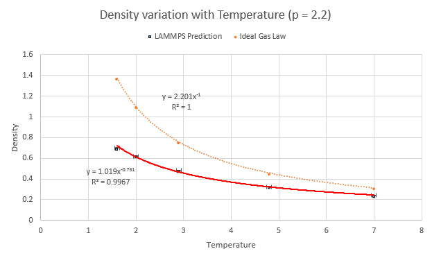
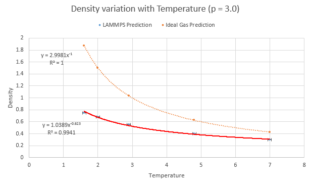
The values of density and temperature output by the computer were plotted alongside the predicted variation of density according to the ideal gas law along with error bars of the standard deviation. The LAMMPS model prediction has an obvious difference in that the values of density are a lower than that predicted by the ideal gas law. This discrepancy increases with increasing pressure and is due to the differences the simulation method has with the ideal gas law. The particles in an ideal gas do not have any ranged attractive/repulsive interactions between themselves whilst the LAMMPS software was instructed to use Lennard-Jones interactions.
NJ: In fact, the ideal gas particles don't interact at all.
The repulsion term in the LJ potential is then responsible for the lower-than-ideal density as the particles push away from each other in the simulation. For higher values of pressure where they are even closer together, the force they experience is larger due to the r-6 relationship of the repulsion- thus a higher discrepancy is seen.
NJ: Can you explain the trend with temperature?
Using LAMMPS to predict heat capacities
Setting up the input file
Fluctuations of a system whose energy is at constant temperature are indicative of the matter's heat capacity. This is related by the following equation:
Where the numerator of the fraction is the variance in the total energy. The input file used in the previous section were modified for a NVE ensemble at different material densities. It now instructs LAMMPS to create the lattice of atoms, melt it to equilibrium and then measure the thermodynamic properties. The average heat capacity is then calculated in the program and output with the rest of the data. Ten copies of the file were made with the following changes in parameter:
- Density = 0.2
- Temperature = 2.0
- Temperature = 2.2
- Temperature = 2.4
- Temperature = 2.6
- Temperature = 2.8
- Density = 0.8
- Temperature = 2.0
- Temperature = 2.2
- Temperature = 2.4
- Temperature = 2.6
- Temperature = 2.8
The content of one of the input files is given below:
Code for the heat capacity calculation
##################################Define Density Variable####################################################
variable d equal 0.8
#####################################################################################
### DEFINE SIMULATION BOX GEOMETRY ###
lattice sc ${d}
region box block 0 15 0 15 0 15
create_box 1 box
create_atoms 1 box
### DEFINE PHYSICAL PROPERTIES OF ATOMS ###
mass 1 1.0
pair_style lj/cut/opt 3.0
pair_coeff 1 1 1.0 1.0
neighbor 2.0 bin
### SPECIFY THE REQUIRED THERMODYNAMIC STATE ###
variable T equal 2.4
variable p equal ...
variable timestep equal 0.0025
### ASSIGN ATOMIC VELOCITIES ###
velocity all create ${T} 12345 dist gaussian rot yes mom yes
### SPECIFY ENSEMBLE ###
timestep ${timestep}
fix nve all nve
### THERMODYNAMIC OUTPUT CONTROL ###
thermo_style custom time etotal temp press
thermo 10
### RECORD TRAJECTORY ###
dump traj all custom 1000 output-1 id x y z
### SPECIFY TIMESTEP ###
### RUN SIMULATION TO MELT CRYSTAL ###
run 10000
unfix nve
reset_timestep 0
### BRING SYSTEM TO REQUIRED STATE ###
variable tdamp equal ${timestep}*100
variable pdamp equal ${timestep}*1000
fix nvt all nvt temp ${T} ${T} ${tdamp}
run 10000
reset_timestep 0
##################################changing ensemble###################################################
unfix nvt
fix nve all nve
#####################################################################################
### MEASURE SYSTEM STATE ###
thermo_style custom step etotal temp press density atoms vol
variable dens equal density
variable dens2 equal density*density
variable temp equal temp
variable temp2 equal temp*temp
variable press equal press
variable press2 equal press*press
variable etot equal etotal
variable volume equal vol
variable esquared equal etotal^2
fix aves all ave/time 100 1000 100000 v_dens v_temp v_press v_dens2 v_temp2 v_press2 v_etot v_esquared v_volume
run 100000
variable avedens equal f_aves[1]
variable avetemp equal f_aves[2]
variable avepress equal f_aves[3]
variable errdens equal sqrt(f_aves[4]-f_aves[1]*f_aves[1])
variable errtemp equal sqrt(f_aves[5]-f_aves[2]*f_aves[2])
variable errpress equal sqrt(f_aves[6]-f_aves[3]*f_aves[3])
variable avenrg equal f_aves[7]
variable avesquarednrg equal f_aves[8]
variable avgvol equal f_aves[9]
variable numatoms equal atoms
variable avenrgsquared equal ${avenrg}*${avenrg}
variable variation equal ${avesquarednrg}-${avenrgsquared}
variable tempsquared equal ${avetemp}*${avetemp}
##########################################Define heat capacity variable###########################################
variable hcapa equal ${numatoms}*${variation}/${tempsquared}
#####################################################################################
print "Averages"
print "--------"
print "Density: ${avedens}"
print "Stderr: ${errdens}"
print "Temperature: ${avetemp}"
print "Stderr: ${errtemp}"
print "Pressure: ${avepress}"
print "Stderr: ${errpress}"
print "Heat Capacity: ${hcapa}"
print "Average Volume: ${avgvol}"
Analysing the data from the output
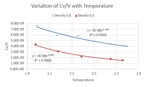
The data output was imported into a spreadsheet processing software. was plotted as a function of temperature for each pressure and both graphs were superimposed for each density. Both graphs exhibited the same trend of a decrease in heat capacity per volume with temperature, but the plot for the density of 0.2 was lower down. The plots were fitted with exponentially and their equations determined to give:
NJ: Why did you make an exponential fit?
- Density 0.2: with an R-squared of 0.9906
- Density 0.8: with an R-squared of 0.9569
It can be seen that a reduction in density results in a lower heat capacity- this is expected and can be explained in terms of the particles involved.
A lower density means less particles per unit volume. Since each particle in the system contributes toward the heat capacity it makes sense that having less particles means a lower contribution and so the term decreases with decreasing density.
NJ: Yes, CV is extensive.
The heat capacity can also be seen to fall with temperature: this is known as the Schottky anomaly and is because of a peak in heat capacity (not seen in graph, the section being visualized is the decrease after the maximum). At a temperature of zero, all the atoms in the system are said to be in their lowest vibrational energy level and the entropy is very low (zero at 0 K) because any transition to higher energy levels is unlikely. The entropy can be increased by increasing the temperature and the effect of temperature on entropy at low temperatures is greater than the effect at higher temperatures. When the temperature provides an energy which is very close to the energy gap between vibrational energy levels, the probability of excitation depends even more on the temperature. At very high temperatures, most vibrational energy levels are populated evenly and so there is only a small change in entropy per change in temperature and so by the relationship:
NJ: The Schottky anomaly really only occurs in solids, but this is a great effort at explaining something without a really satisfying answer. Well done.
The heat capacity thus decreases when temperature increases, as it gets harder to excite the atoms to higher vibrational energy levels.
NJ: Wrong way around - if it's harder to excite atoms, the heat capacity increases.
Radial distribution functions of Lennard-Jones matter
Running, collecting and analysing data
The software Visual Molecular Dynamics (VMD) contains a function which can calculate the average radial distribution of atoms about other atoms. This method was deployed on three input files with varying values of density and temperature to represent extremes of a solid (of crystal type fcc), liquid and vapor on the Lennard-Jones coexistence curve. Their values are as follows:
- Solid (fcc)
- Density: 1.2
- Temperature: 1.0
- Liquid
- Density: 0.4
- Temperature: 0.8
- Vapor
- Density: 0.2
- Temperature: 2.0
NJ: Your liquid density is probably in the coexistence region, unfortunately. Something like rho=0.8 would be better.
NJ: Your vapour isn't vapour, it's supercritical fluid. The temperature should be below about 1.2 in this case.
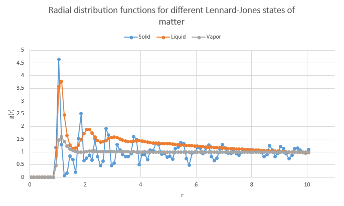
Their radial distribution functions were calculated in VMD and the graphs superimposed in a spreadsheet processing software. Though not shown, the number of particles in the solid and liquid simulations were equivalent (3375).
The differences between the states of matter on the plot are immediately visible. The graph of the solid matter has the sharpest and highest peaks of the three and this is because the probability of finding a particle at a certain distance in an ordered lattice is very high- the maxima in the plot corresponds almost exactly to the positions of neighboring atoms and useful information, such as the lattice spacing, can be extracted from the plot with ease. This "erratic" graph behavior continues along the graph as atoms are always in localized positions which will show as peaks. The liquid graph has two main differences from that of the solids:
- The maxima appear at lower values of g(r)
- There is a lower probability of finding atoms at specific positions in a "lattice formation" in a liquid (correlating to the maxima) as the structure is more random due to the ability of the particles to move. Atoms are more likely in this simulation to be found in random places than in the computation of the solid and so at higher values of r, the graph begins to taper off linearly without much fluctuation to a constant value of 1 which represents the average density at large ranges. This suggests random movement, and hence placement, of particles in this simulation.
- The peaks are rounded off instead of sharp
- Whilst there is a higher degree of disorder in a liquid than a solid, there is still some structure due to the inter-atomic attraction forces of the Lennard-Jones and so the radial distribution still displays maxima of likely atomic positions. However, due to the ability of atoms to move around more freely than in a solid, the distances at which they may be located deviate and so a rounded maxima accounts for this.
The vapor exhibits similar properties to the liquid except for the presence of only one maxima- this is due to the attractive Lennard-Jones interactions between the particles that causes "clusters" of atoms where they have relatively low internuclear distances. At high values of separation, the distribution appears constant due to the random movement of particles, much like the case for the liquid.
NJ: We generally classify the phases as follows: gas, no order; liquid, short range but no long range order; solid, short and long range order.
Analysing the plot for a solid Lennard-Jones material
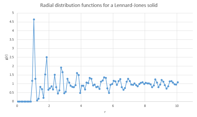
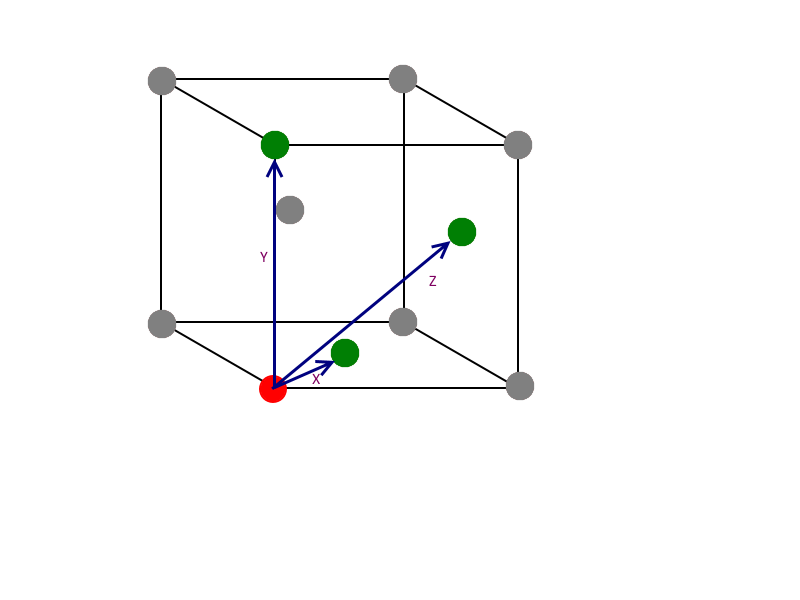
The radial distribution for a Lennard-Jones solid is shown above. From r = 0 to ~0.85, there is no distribution as this is either within the atomic radius of the atom being considered, or too close that any particle in this area would be repelled away. Keeping in mind that the solid structure is face-centered cubic (fcc), the first large peak at r = 1.05 corresponds to the very next neighbors. As a larger distance is considered, the two peaks after that, at r = 1.45 and 1.85 are due to the consecutive neighbors. These are shown below, labelled X, Y and Z from smallest to largest:
It can be seen from the diagram that X corresponds to r = 1.05, as the atom responsible is the shortest distance away. Y is responsible for r = 1.45 and Z for r = 1.85. Inspection of the picture also shows that Y is the same as the lattice dimensions, so the lattice spacing is equal to 1.45 reduced units.
NJ: You should get the same answer that you worked out earlier, about 1.49. It won't be exact because it's tricky to read off the graph. You could, however, use the three lattice distances and compare them to the graph, get three values for a, and then average.
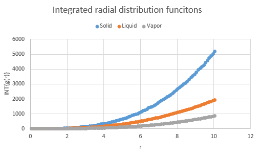
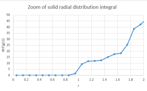
The integration of the radial distribution functions of the phases are also shown, along with a zoomed version for the solid which is useful for calculating the coordination number:
Calculating the areas under the respective peaks from zero gives the number of atoms within that radius. For example, the peak at r = 1.05 actually "ends" at r = 1.25. Using the integral graph, reading off this point yields the area and hence the atom count up to that point. Using this method, it was determined that:
| Peak at | Area | Atom Count |
|---|---|---|
| X | 12.0132 | 12 |
| Y | 18.4429 | 18 |
| Z | 42.2626 | 42 |
The atom count shows cumulative results, so subtracting X from Y and Y from Z yields the number of atoms at that radius away.
- X coordination 12
- Y coordination 6
- Z coordination 24
Indeed the coordination for a face-centered cubic lattice is 12 and so the radial distribution shows that the simulation is in line with real world results.
NJ: Excellent
Calculating Diffusion coefficients
The following simulation uses these parameters for setting up solid, liquid and vapor phases states (except for the cases of one million atoms, in which the parameters were not known):
- Solid (fcc)
- Density: 1.2
- Temperature: 1.0
- Liquid
- Density: 0.4
- Temperature: 0.8
- Vapor
- Density: 0.2
- Temperature: 2.0
Mean Squared Displacement method
The mean squared displacement (MSD) is a measure of the degree of random motion and when applied to atoms in this simulation, give an indication as to how much space has been "explored". It is conveniently related to the diffusion coefficient by the following equation, which can be rearranged and integrated:
NJ: Yes, it's nice to show this - what is c though?
The gradient of the line of best fit on an MSD against time graph can therefore be divided by six to yield the diffusion coefficient.
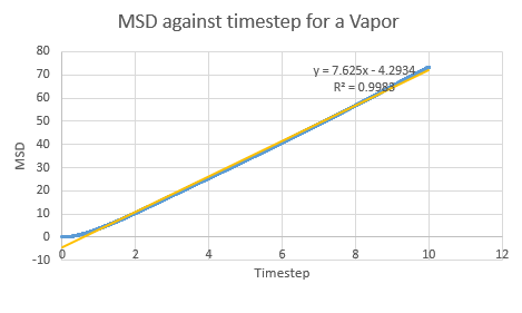
In a chaotic substance such as the Lennard-Jones vapor, the MSD is very high as the particles move about randomly and occupy as much space as possible- thus it is expected that the MSD would increase with time (keeping in mind that the starting positions for all the particles in the simulation is in a well ordered lattice). Indeed this is what is seen on a plot for a vapor:
NJ: Can you explain the curvature at the start of the vapour curve?
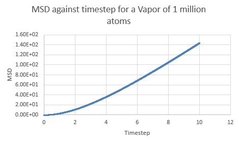
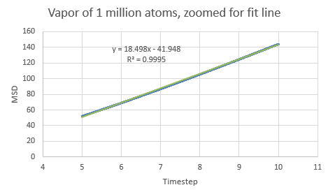
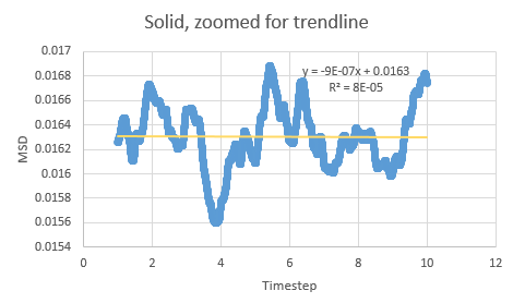
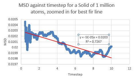
If the linear section of the one million atom vapor plot is considered (which corresponds to the system reaching equilibrium), a line of best fit can be added:
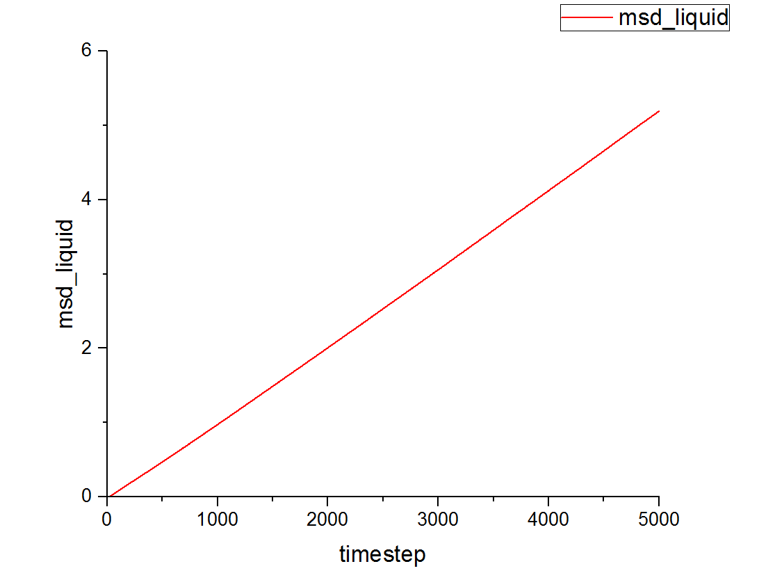
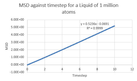
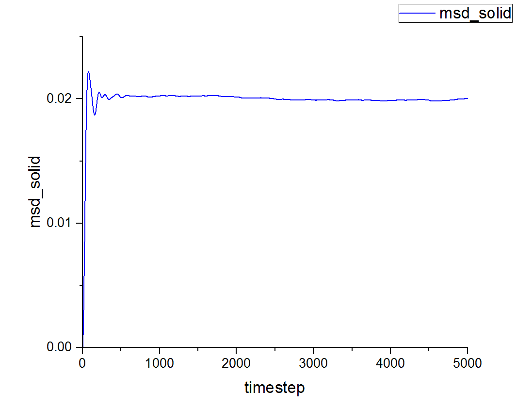
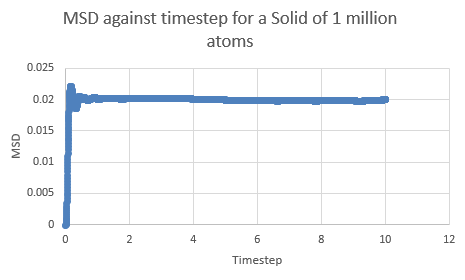
This can be contrasted with the MSD against time graphs for the solid and liquid phases as well:
This is a trend that is expected- in the case of the one million atom simulations, it can be seen that the solid MSD reaches a maximum at about 0.022 whilst the liquid and vapor reach MSD values of approximately 5 and 140 respectively. This is indicative of the atomic motion within the systems as the low MSD value for solids shows that they do not move very far from their original points- and this makes sense as the atoms in a solid are locked at fixed points at which they can only vibrate slightly about. Contrasting this to the liquid and vapor plots, which have higher MSD values and show the ability for the atoms to actually move about and interchange positions with one another.
The table below shows the data extracted from each simulation, where simulations tagged (1M) are the one million atom runs:
| Simulation | Gradient | Diffusion Coefficient |
|---|---|---|
| Solid | ||
| Solid (1M) | ||
| Liquid | ||
| Liquid (1M) | ||
| Vapor | ||
| Vapor (1M) |
Between the simulations, the diffusion coefficient for the solids are effectively zero- which agrees with real life observations as stable solids are not known to diffuse in any feasible span of time. The negative gradients seen are due to fitting of the line rather than any physically significant interactions between atoms.
NJ: Why do you think the liquid and vapour values differ between the 1M atom results and your own?
Velocity Autocorrelation Function method
Velocity Autocorrection (VAC) is a way of measuring the correlation between the velocities for randomly moving bodies in a system. If the particles in the simulation are truly moving randomly, then their VAC will be at a minimum as there is no correlation between their movements. The function itself can be denoted as:
Where t is the time and is the timestep being considered for calculation. This can also be written as integrals of the velocities:
From the earlier sections, it is said that the position of a simple harmonic oscillator could be defined through trigonometric functions. Knowing as well that velocity is the first differential of displacement, the following derivation can take place:
Using the trigonometric identity that :
This can be integrated and split up like so:
The functions that are invariant with respect to t are then taken out of the integral:
This expression is placed back into the equation for ...
...and like terms cancelled out:
The term is an odd function (as it arises from the product of an odd sine function with an even cosine function, and odd times even makes odd) and so is antisymmetric about the y axis. Integrating such a thing from negative infinity to infinity will thus result in an answer of zero, as the areas effectively "cancel out":
So a function for the VAC has been deduced for a system in simple harmonic oscillation.
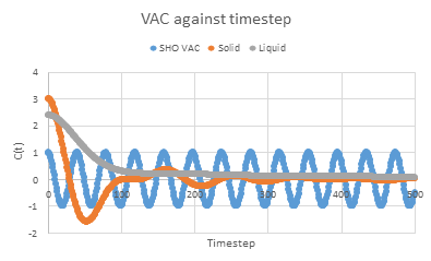
A plot of the VAC function against timestep was made for solid and liquid phases. These were superimposed with the graph for shown below:
The minima in the VAC functions represent the times where there was a negative correlation between the velocities of all the atoms in the system. When the atoms are first placed in the simulation, they are positioned neatly in a lattice.
NJ: This is an interesting idea, but the "lattice melting" section isn't included in this data.
Upon starting calculations, they begin to move towards each other due to the attractive interatomic forces, and this is shown as the high value at which each plot starts at- however as they get closer the repulsive force between them also increases which in turn lowers their velocity. At some point, the atoms are close enough that they begin to repel more than pull in and so they move away from each other- creating a minima in their VAC functions. Eventually, when the system is in equilibrium, there is no correlation between the atomic velocities as they are moving randomly and being influenced by the forces of basically every other atom in the system and the plots settle at zero.
NJ: The minima effectively correspond to collisions between atoms. In the liquid, the minimum corresponds to collisions with the "solvent cage".
The difference between the liquid and solid VAC functions is that the solid graph tends to fluctuate more, with more minima and maxima present whilst the liquid graph quite steadily approaches zero. In a solid, the particles are bound to certain points and so can only vibrate in place. This creates a rigidity in their movement that is shown by the more erratic changes in the respective VAC function. In the case of a liquid, the atoms may freely move and mingle with each other- there is no restoring force that makes it move back to a particular point and so there is a smooth decrease in velocity correlation as the atoms shift past one another- almost having a "damping" or attenuating effect on their changes in velocity.
The harmonic oscillator VAC function is different to the solid and liquid plots due to its simplicity as a system and its intrinsic considerations- the harmonic oscillator models a particle that when moved from an equilibrium position experiences a restoring force in the opposite direction, proportional to its displacement. The function that was deduced earlier for the oscillator does not consider external forces- such as the other many atoms in the simulation which also impart both attractive and repulsive forces to distort the plots.
NJ: Good
The diffusion constant can be calculated from the VAC functions by the relationship:
This tells us that dividing the area under the graph of VAC against time from zero to infinity by three will give the diffusion coefficient. In order to calculate the area, the trapezium rule was used. The plots of integral and running integral over time are given below for all systems, with the plateaus of the running integrals being the area under the graph:
These yielded the following data:
| Simulation | Area | Diffusion Coefficient |
|---|---|---|
| Solid | ||
| Solid (1M) | ||
| Liquid | ||
| Liquid (1M) | ||
| Vapor | ||
| Vapor (1M) |
NJ: How do these compare to the results from the MSD?
The largest source of error in using this method arises from the use of trapeziums to calculate the area. In this case, one trapezium per timestep was used (effectively calculating the area between timesteps). The number of trapeziums used can greatly affect how well the true area can be resolved and a higher degree of accuracy can be attained by considering a trapezium every half time step rather than every whole timestep.
