Talk:Mod:ThirdyearPSRWliquidsimulationsexp

JC: General comments: This is an excellent report, well done. You have given a good answer to each task and very thorough explanations, backed up by additional references.

Introduction to Molecular Dynamics Simulation

The aim of this report is to demonstrate how Molecular Dynamics can be used as a powerful tool to model a simple Lennard-Jones fluid initially in the canonical ensemble [N, V, T] and then subsequently in the isobaric ensemble [N, P, T]. The systems modelled are entirely classical which is why MD, a simple stochastic method is used. The simulations involved will utilize periodic boundary conditions when choosing a simulation box containing N atoms; assigning each atoms initial positions and velocities such that the system is as close to equilibrium as possible (this is a result of comparing the total kinetic energy to the equipartition principle), and finally measuring any desired thermodynamic quantities. Monitoring a system's velocities and computing the total kinetic energy is computationally costly, however algorithms such as the Velocity-Verlet (used extensively in this report), use a neighbouring list technique which reduces the time taken. Short references to the underlying theory will be invoked and simulations of the vapour, liquid, solid and super-critical states of the fluid will be modelled, its limitations discussed, and this will be compared to the as the equation of state/ideal gas model. Finally Radial Dstribution Functions (RDF's) and Velocity Autocorrelation Functions (VACF's) of each phase will be analysed and structural properties identified.

Tasks 1, 2 and 3- The Velocity-Verlet algorithm vs. Analytical simple harmonic oscillator

We consider the 1D classical harmonic oscillator limiting case; We shall observe the system where the angular frequency ω = 1.0 and phase factor ϕ = 1.0. The particle position x(t) is given by the following formula;

$x\left(t\right)=A\cos (\omega t+\varphi )$

Data from the file 'HO.xls.' was retrieved and contains three columns.

1. ANALYTICAL- the exact value for the velocity v(t) for the classical harmonic oscillator
2. ERROR- the absolute error between the analytical and velocity-varlet solution
3. ENERGY- the total energy for the classical harmonic oscillator determined from Velocity-Verlet results

The initial time-step given in the file was 0.1. The total energy for the harmonic oscillator is given by its time-dependent kinetic and potential energy contributions specified in the formula;

$E=K(t)+U(t)=\frac{1}{2}m{v}^2(t)+\frac{1}{2}k{x}^2(t)$

The results for the position and total energies as a function of time are shown in the gallery below.

• 
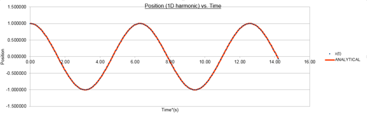  figure 1; position as function of time for the analytical harmonic oscillatorr and the Velocity-Verlet Algorithm, Δt=0.1
• 
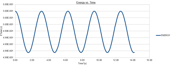  figure 2; Velocity-Verlet Total Energy vs. Time, Δt=0.1

The positions calculated by the analytical harmonic oscillator and the Velocity-Verlet algorithm are the same. These values of position x(t) were then inputted into algorithm and the total energy was computed using equation (2). The total energy of an isolated simple harmonic oscillator should remain constant and only the individual kinetic and potential energy contributions vary. The Velocity-Verlet algorithm utilises molecular dynamics based upon simple Newtonian Mechanics to calculate a trajectory of the oscillating particle. However classical mechanical variables such as velocity are time-reversible and continuos in time and space whereas the variables in the algorithm have been discretised. Despite this difference it is observed that the mean energy should still be conserved in the discrete mechanics utilised in our the simulation and as such one of the key tests of accuracy for these trajectories is that the conservation of energy principle should be upheld and the total energy should hold a constant value. From figure 2 we can see the total energy follows a cosinusoidal function about an average value of 0.499 in reduced units with a maximum percentage error of 0.2%.

JC: The Velocity Verlet algorithm has time-reversal symmetry.

• 
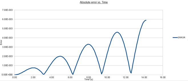  figure 3; Absolute error as a function of time, Δt=0.1
• 
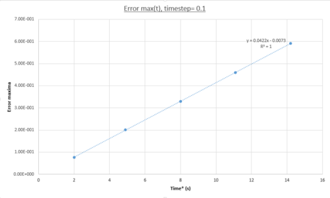  figure 4; Error maxima as a function of time, Δt=0.1

From figure 3 is it seen that the absolute error between the analytical harmonic oscillator and that determined by the Velocity-Verlet algorithm is both periodic

NJ: Not periodic - periodic means $x(t)=x(t+T)$, for some period T.

and increases in magnitude with time. The maximum error of the algorithm increasing as a function of time because the trajectory used is calculated by iteration. This could be better visualized in [x(t), v(t)] phase-space where the analytical periodic solution would appear as a circle NJ: ellipse, but the Velocity-Verlet solution would appear similar to a Fibbonaci expansion, increasingly determining a trajectory with more deviation after each time-step. At each time-step a new trajectory point is established using the previous one and as such errors are compounded and increase with the number of time-steps simulated. The increase in maximum error is quantified in figure 4 by isolating each peak in figure 3 producing a linear plot. The straight line equation %E_max(t) = 0.0422t - 0.0073 demonstrates this behaviour. The periodicity can be explained simply by taking into account the periodic energy of the system and as such the errors incurred in the MD trajectory used by the algorithm at nearly periodic time spacing will still calculate the exact same energy as the analytical solution.

• 
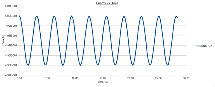  figure 5; Velocity-Verlet Total Energy vs. Time, Δt=0.1

Experimenting with different values of the time-step in the Velocity-Verlet algorithm demonstrates that a more accurate iteration is achieved when a smaller time-step is used. Figure 5 shows the total energy as a function of time when this increases to 0.2, the maximum deviation in the total energies calculated over the simulation was 1.0%. Therefore using a time-step of less than 0.2 is required to keep the maximum deviation under this value, the importance of this is such that the simulation obeys the conservation of energy as discussed before and a more accurate average value will be simulated.

NJ: Excellent, very thorough presentation.

Task 3- The Lennard-Jones Potential

The equation for the empirical Lennard-Jones two body interaction potential is;

$V(r)=4\epsilon [{\left(\frac{\sigma }{r}\right)}^{12}-{\left(\frac{\sigma }{r}\right)}^6]$

The potential is characterized by a steep repulsion at internuclear distances ≤ σ, where σ is the radial distance between the two bodies in direct contact. The potential also consists of a favourable potential well characterized by its well-depth -ε, and its asymptotic behavior whereby the potential V(r) →0 as r→∞.

The relationship between a force and its corresponding Lennard-Jones potential is given by;

$\mathbf{F}=-\frac{V\left(r\right)}{\mathrm{d}\mathbf{r}}=4ϵ(12{\sigma }^{12}{r}^{-13}-6{\sigma }^6{r}^{-7})$

1.To find the equilibrium seperation this derivative is set equal to zero and the corresponding equation solved for r. The working is as follows;

$4ϵ(12{\sigma }^{12}{r}^{-13}-6{\sigma }^6{r}^{-7})=0,\frac{12{\sigma }^{12}}{r^{13}}=\frac{6{\sigma }^6}{r^7}$

Simple equating of terms and rearrangement yields the solution $r_{eq}=2^{\frac{1}{6}}\sigma$

2. To find the potential at equilibrium (well-depth), of which will be a stable minima, is achieved by substituting $r_{eq}$ into our original equation for the Lennard-Jones potential.

$4ϵ(12{\sigma }^{12}(2^{\frac{1}{6}}\sigma {)}^{-12}-6{\sigma }^6(2^{\frac{1}{6}}\sigma {)}^{-6})=4ϵ(\frac{1}{4}-\frac{1}{2})=-ϵ$

3. To find the separation $r_o$ where the Lennard-Jones potential is equal to zero, the LJ potential equation set equal to zero, then dividing by ε, equating the resultant terms and solving for r. This yields the solution $r_0=\sigma$.

4. The corresponding force at this internuclear separation is found by substituting $r_0=\sigma$ into the original $\mathbf{F}=-\frac{V\left(r\right)}{\mathrm{d}\mathbf{r}}$ equation.

This yields $\mathbf{F}=-4ϵ(12{\sigma }^{12}{\sigma }^{-13}-6{\sigma }^6{\sigma }^{-7})$, where the σ's, excluding one on the denominator for each term cancel, by rearrangement $\mathbf{F}(r_0)=\frac{24ϵ}{\sigma }$

5. The following integrals are evaluated where σ = ε = 1.0 such that $V(r)=4\epsilon [r^{-12}-r^{-6}]$

• $\underset{2\sigma }{\overset{\mathrm{\infty }}{\int }}V\left(r\right)\mathrm{d}r=4\underset{2\sigma }{\overset{\mathrm{\infty }}{\int }}[r^{-12}-r^{-6}]\mathrm{d}r=4{[-\frac{r^{-11}}{11}+\frac{r^{-5}}{5}]}_{2\sigma }^{\mathrm{\infty }}=-0.0248$
• $\underset{2.5\sigma }{\overset{\mathrm{\infty }}{\int }}\varphi \left(r\right)\mathrm{d}r=-0.0082$
• $\underset{3\sigma }{\overset{\mathrm{\infty }}{\int }}\varphi \left(r\right)\mathrm{d}r=-0.0033$

NJ: Very good

Task 4 and 5- Periodic Boundary Conditions for MD simulations

An example physical system looking to be modelled consists of 1ml of water under standard conditions- T = 298.15K, P= 10⁵Pa.

The Molecular weight of water = 18.015gmol^-1 and under standard conditions has a density ρ = 0.9970gml^-1, therefore in 1ml there is 1g of water.

Therefore the number of molecules of water in 1ml is calculated;

$n=\frac{m}{Mr}=\frac{1.00g}{18g.mo{l}^{-1}}=0.056mol$ and therefore no.molecules N = 0.056mol * 6.023x10²³mol^-1 = 3.343x10²²

Calculating the volume of 10000 molecules of water under standard conditions;

$m=\frac{\rho }{V}=nMr=\frac{10000Mr}{Na}$therefore by rearrangement it is found that V = 2.983x10^-19ml^-3

During all the MD simulations carried out in this report periodic boundary conditions (PBC's) are applied. This is because it is not possible to simulate realistic volumes of fluids as these contain nN_A numbers of molecules and therefore the same number of individual Newtonian dynamic second order linear differentia equations to compute. Because of this PBC's are chosen to approximate large bulk system behaviour. PBC's utilise a minimum image and a repeated zone of which is repeated in every translational axis about a simulation box. A given molecule A will interact with all other molecules inside the the simulation box, generally equating to 10^1-2 pair-wise interactions. This reduces the computational time needed for simulation. The use of a repeated zone also means that molecules that would have been near the simulation box walls don't have a perturbed fluid structure. The system is feasible because if a molecule leaves the simulation box another identical molecule enters on the opposite side such that the total number is constant.

An example to demonstrate PBC's in a cubic simulation box which runs from $(0,0,0)$ to $(1.0,1.0,1.0)$ is for an atom A at starting position $(0.5,0.5,0.5)$ in that travels along a vector path defined by $(0.7,0.6,0.2)$.

As soon as the atom hits the boundary of the simulation box in the x and y directions it is immediately reflected onto the opposite side of the box. This effect is orthonormal along the axes and as such the atom never encounters the z-face. Therefore at the end of the time-step the final position of the atom is $(0.2,0.1,0.7)$.

Task 6- Reduced Quantities

In all the MD simulations conducted in this report reduced quantities are utilised to make data value magnitudes more manageable. This various reduced quantities are calculated by division by a known scalar for example;

distance $r^{*}=\frac{r}{\sigma }$  energy $E^{*}=\frac{E}{ϵ}$ temperature $T^{*}=\frac{k_{B}T}{ϵ}$

For example Argon;

• $\sigma =0.34nm$

• $\frac{ϵ}{k_B}=120K$ therefore the well-depth = 1.656x10^-24KJ = 0.998KJmol

• $r_c^{*}=\frac{r_c}{\sigma }$ therefore the Lennard-Jones cutoff point $r_c$ = 1.088nm in real units

• $T^{*}=1.5$ therefore using the value for the well depth $ϵ$ calculated, the temperature in real units is equal to $T=\frac{ϵT^{*}}{k_B}$ = 180K

A note on the LJ-cutoff point: When carrying out MD simulations it is advisable to truncate the inter-nuclear distance of interaction to avoid an excessive number of pair-wise interactions being simulated.

$V_{{LJ}_{trunc}}(r):=\{\begin{array}{ll}{V}_{LJ}(r)-V_{LJ}(r_c)& \text{for }r\le r_c\\ 0& \text{for }r>r_c.\end{array}$

This is both useful to save computational time and is justified because the LJ r^-12(repulsive) and r^-6 attractive terms both decay rapidly as r increases. The truncated LJ potential is achieved via a cutoff distance r_c, generally around the magnitude of 2.5σ as this is approximately equivalent to $\frac{1}{60}$ of the minimum potential well-depth of -ε. Therefore after this cutoff distance the pair-wise interaction can be considered insignificant within the precision of the simulations undertaken and are assigned a value of 0. Furthermore a jump dicontinuity in the potential energy is avoided as the LJ is shifted upward such that at the cut-off radius it is exactly equal to zero.

NJ: Actually, we're not doing that. It is common though, well researched. The shifted version is usually called the "truncated and shifted LJ potential".

Equilibration

Task 1 and 2- Choosing initial atomic positions

The MD simulations run using the Velocity-Verlet algorithm require a trajectory to be calculated for each individual particle. This therefore requires the computation of the same number of second order linear differential equations such that each is an initial value problem. When modelling a solid system this is easily done by using knowledge of a crystals lattice structure and motif and then using its inherent infinite translational symmetry.

For example considering a simple primitive cubic lattice where each equivilent lattice vector/unit cell side length x,y and z = a = 1.07722 in reduced units, atomic positions lie on each edge of the cell. As a result the volume of the unit cell is 1.07722³ = 1.25. Each simple cubic lattice unit cell contains the equivalent of 1 atom due to sharing with neighboring cells and therefore the density of the cell;$\rho =\frac{1}{1.25}=0.80$

An FCC (face-centered cubic) lattice on the other hand contains the equivalent of 4 atoms per unit cell. If such a crystal had an intrinsic density of 1.2 the lattice vectors can be calculated as follows;$\rho =\frac{4}{a^3}=1.20$ therefore $a=1.494.$

When calculating trajectories of solid crystalline systems an input file containing the following lines is used:

region box block 0 10 0 10 0 10
create_box 1 box

This creates an orthogonal geometric region, the simulation box, a cube consisting of 10 lattice-spacing's along each axis. This corresponds to a box of 1000(10x10x10) unit cells, 10 along each Cartesian axis, and therefore in the case of a cubic lattice will contain 1000 lattice points which will be filled with atoms later. Analogously as mentioned before an FCC lattice unit cell contains four times as many atoms per unit cell so upon the same treated in the input file 4000 lattice points would be generated and 4000 atoms simulated.

• 
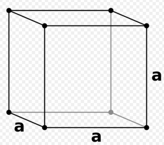  figure 6; Primitive cubic lattice unit cell, lattice vector a
• 
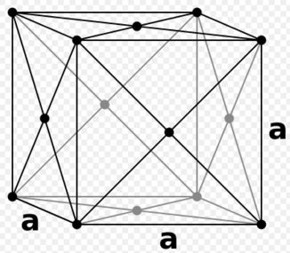  figure 7; Face-centered cubic lattice unit cell, lattice vector a

However for this report a Lennard-Jones fluid with no long-range order or single reference cell for the simulation box is modelled. It is possible to simply compute random atomic starting coordinates in the simulation box. However this can cause major problems for the resulting time-evolving trajectories especially in large/dense systems where there would be a large probability of two atoms initially being positioned within each-others excluded volume such that r_AB<σ. The resulting initial overlap is catastrophic especially for a LJ-fluid because of its very strong short-range repulsive term. The subsequent system energy would increase rapidly and would be highly unrealistic and lead to large errors which could not be rectified. This is analogous using a time-step that is too large as similar highly repulsive interactions would occur over time. The initial configurations are crucial as the system is only simulated for a short time frame and therefore a starting configuration close to equilibrium needs to be ensured for an accurate MD simulation i.e. need to start near a local PE minima.

Task 3 and 4- Setting atomic physical properties

Using the LAMMPS manual the following input file lines of code are explained:

mass 1 1.0

The command 'mass' sets the mass for all the atoms (≥1 types).

General syntax: 'mass I value': where I- atom type and value- mass.

Therefore 1 specifies there is only one atom type in the lattice and 1.0 species the mass values of all of these atoms as unity.

pair_style lj/cut 3.0

The command 'pair_style' sets the formula(s) LAMMPS uses to compute pairwise interactions. LAMMPS pairwise interactions are defined between atomic pairs within a cutoff distance as discussed before, generally r_c≈2.5σ, this cutoff can take an arbitary value smaller of greater than the simulation box dimensions. The function therefore sets the active interactions which evolve with time.

General syntax: 'pair-style style args': where style- one of the styles/pairwise potentials in LAMMPS and args- arguments used by that particular style.

Therefore lj/cut specifies a Lennard-Jones potential with a cutoff at 3.0σ and no Coulombic potential.

pair_coeff * * 1.0 1.0

The command 'pair_coeff' specifies the pairwise force field coefficients for one/more pairs of atom types, with the number and meaning being dependent on the pair_style chosen. The command is written after the pair_style command and modifies the cutoff region for all atomic pairs such that it holds for the entire LJ potential computed.

General syntax: 'pair_coeff I J args': where I,J- specify atom types and args- coefficients for ≥1 atom types

In the line of code used ' * * ' specifies no numerical value and that all atom pairs within the lattice (n→N) are to be specified and 1.0 1.0 specifies the LJ force field coefficients.

NJ: What do you mean by coefficients?

In the MD simulations the Velocity-Verlet integration algorithm is utilized as the $X_i(0)$ and $V_i(0)$ are specified in the initial value problem. Specifying the initial velocity is easy as simulations will occur at thermodynamic equilibrium and as such obey Maxwell-Boltzmann statistics. This is computed by choosing random velocities where the total CoM = 0 and re-scaling to fit the desired system temperature given by statistical mechanics and the equipartition principle in the classical limit.

Task 5- Monitoring thermodynamic properties

When running MD simulations it is useful to monitor how properties change dependent on the time-step trajectories are calculated from. It is therefore useful to code the input file using following the second chunk of code compared to the first.

1)

timestep 0.001
run 100000

2)

### SPECIFY TIMESTEP ###
variable timestep equal 0.001
variable n_steps equal floor(100/${timestep})
variable n_steps equal floor(100/0.001)
timestep ${timestep}
timestep 0.001

### RUN SIMULATION ###
run ${n_steps}
run 100000

This is because the timestep can be stored as a varible, which is then used in the 3rd line second line of code. This line allows for the different timesteps to simulate for exactly the same overall time in reduced units. For example, setting n_steps equal to 100/timestep tells LAMMPS to simulate for one-hundred thousand steps, when the variable is set to 0.001 and this corresponds to a total time of 100. By analogy for a timestep of 0.002 this would correspond to n_steps = fity-thousand, but crucially the overall time simulated would still be 100. In contrast the first chunk of code would simply simulate for a time equal to the timestep chosen multiplied by the 100000, from the line 'run 100000' and result in different simulation times for different timesteps. This is undesirable as modifying the timestep and comparing results on the same x-axis is crucial to determining the optimum timestep value. Note the floor function is used in case the 100/timestep output is not an integer and rounds this down.

NJ: Nice explanation

Visualizing trajectories

Time evolving MD trajectories are monitored using VMD software. Figures 8 and 9 demonstrate this when applied to a simple cubic lattice at t=0 and then at a later time. Figure 10 shows it is possible to visualize two individual particle trajectories and the PBC's used were clearly seen as atoms dissapeared and reappeared at opposite sides of the simulation box.

• 
  figure 8; simple cubic lattice at t=0
• 
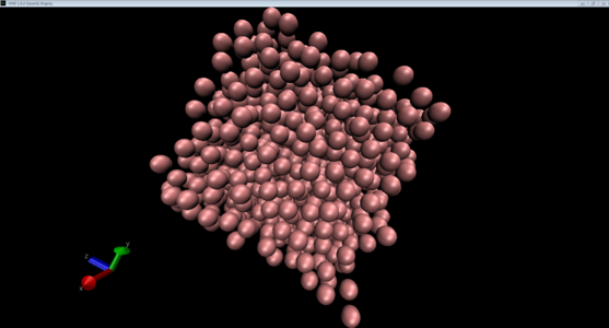  figure 9; simple cubic lattice at t=nΔt=0.1
• 
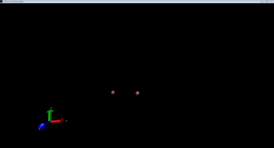  figure 10; simple cubic lattice individual particles at t=nΔt=0.1

Task 6- Checking equilibrium

MD trajectories for Δt=0.001 are calculated and plots for the total energy, pressure and temperature as a function of time are shown below. In all three cases the system reached equilibrium as each thermodynamic property started to fluctuate about a constant average value within the simulation timescale. Due to MD's stochastic nature the values continually fluctuate about these values in a Gaussian fashion. Specifically all these properties reached equilibrium after t=0.3. This is demonstrated by their average values being equal to the linear fit y-intercept.

• 
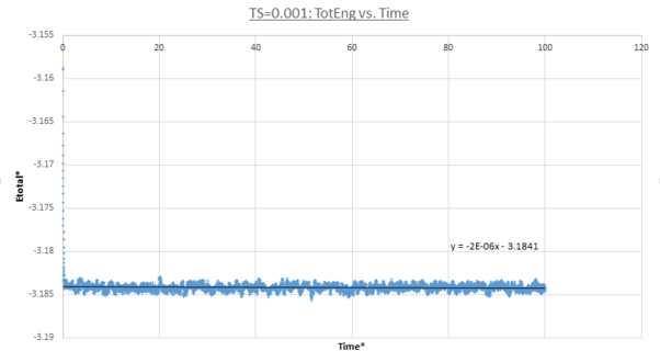  figure 11;Total energy vs. time, Δt=0.001
• 
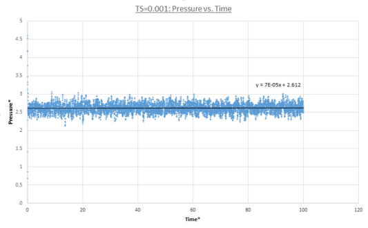  figure 12;Pressure vs. time, Δt=0.001
• 
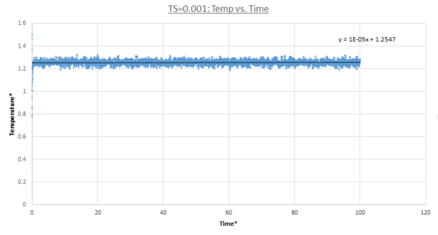  figure 13;Temperaturevs. time, Δt=0.001

Choosing the optimum timestep requires a balance to be struck between computational efficiency when modelling a long timescale, and simulation accuracy. A smaller timescale will reflect the physical reality of the systems pair-wise interactions most accurately. However larger timesteps are useful when modelling trajectories over a longer timescale as less individual computations need to be done for the same overall time-frame. This is quantified:

t𝛕 = nΔt and t_CPU = nΔt_CPU and the computational expense ∝N² with time-step

From figure 14 is can be seen that the time-step 0.015 is a particularly bad choice for the MD simulation as the system never equilibriates and deviates increasingly with time from the standard values obtained with the shorter time-steps. This is because the system is unstable because it permits devastating atomic collisions as the large Δt propagates relative atomic positions where r_AB<σ. This interaction as stated previously generates a severe repulsive force propelling atoms apart and raising the system energy. Over time the occurrence of these interactions continues, explaining the increasingly large deviations. The time-steps 0.01 and 0.0075 do allow the system to equilibriate, but crucially the total energy values this occurs at is larger than that for the remaining two smaller time-steps simulated and therefore do not yield an accurate simulations of the system. As seen before, smaller time-steps lead to more accurate trajectory simulations, reaching a Lennard-Jones potential minima as seen when comparing 0.2 and 0.1, as such these time-steps are also not reliable. The time-steps 0.0025 and 0.0001 both equilibriate at the lowest total energy value, however when taking into account computational efficiency it is found that a time-step of 0.0025 is most useful for subsequent MD simulations.

• 
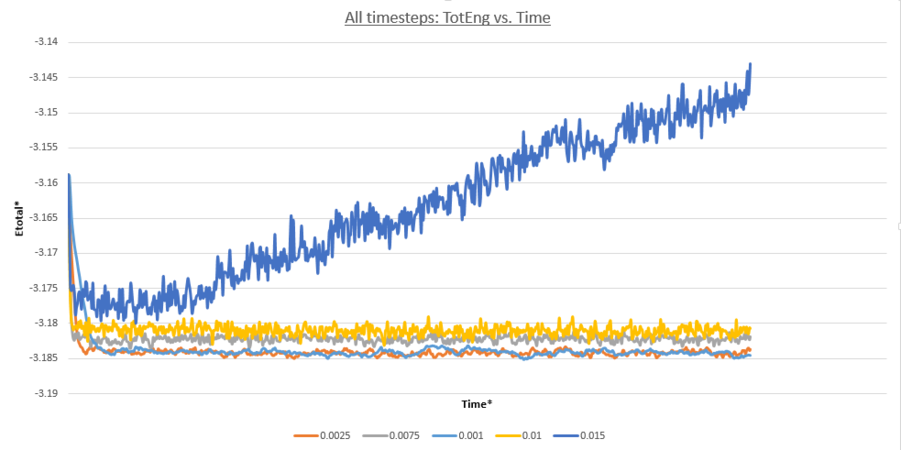  figure 14;Totat energy vs. time, for all timesteps

JC: Good choice of timestep and explanation. Energy should be independent of timestep so the smallest two timesteps can be seen to be the most accurate.

Running Simulations under Specific Conditions

Simulations in this section are run in the isobaric ensemble [N, P, T]. Initial atomic positions are as before where a pseudo-crystal is melted to generate equilibrium-like conditions.

Task 1- Conditions to simulate a LJ fluid

The critical temperature T^* = 1.5 is defined as the temperature above which no value of pressure can cause liquidation and as such the LJ fluid will always be supercritical above this tempeature. Because of this as long as the temperature modelled is greater than equal to T^* , the pressure can be chosen freely. A supercritical fluid is modelled using MD as this is easier to compute as opposed to when the system is in two phases; vapour and liquid which occurs below the critical temperature.

• The temperature chosen are: T₁ = 2, T₂ = 3, T₃ = 4, T₄ = 5, T₅ = 6
• The pressures chosen are: P₁ = 1 and P₂ = 10
• The time-step chosen: Δt = 0.0025 for the reason specified in the previous section

Task 2- Simple correction factors

Controlling the temperature

The equiparition theorem derived from statistical mechanics tells us that each translational DoF of the system contributes $E_K=\frac{3}{2}N{k}_{B}T$ to the total internal energy of the system at equilibrium. Therefore for a total system consisting of N atoms the following equation holds: $\frac{1}{2}\sum _i{m}_i{v}_i^2=\frac{3}{2}N{k}_{B}T$

JC: There are 3 translational degrees of freedom for each molecule, along x, y and z.

Because MD simulation temperatures fluctuate the total kinetic energy of the system and analogously the temperature $T$ can at different time-steps be either larger or smaller than the specified temperature $\mathfrak{𝔗}$ chosen to simulate at. A correction factor $\gamma$ can be introduced to correct this, which is inputted by via multiplication by the velocity.

Two simulataneous equations for the temperature in terms sum of the kinetic energies of individual particles results;

$1)\frac{1}{2}\sum _i{m}_i{v}_i^2=\frac{3}{2}N{k}_{B}T$

$2)\frac{1}{2}\sum _i{m}_i{\left(\gamma v_i\right)}^2=\frac{3}{2}N{k}_B\mathfrak{𝔗}$

To solve these and find gamma at a specified $\mathfrak{𝔗}$ take the LHS of equation 2 and divide by the LHS of equation 1. All terms cancel expect the constant gamma for each individual particle revealing:

${\gamma }^2=\frac{\mathfrak{𝔗}}{T}$ Therefore by rearrangement$\gamma =\sqrt{\frac{\mathfrak{𝔗}}{T}}$

JC: Correct.

Controlling the pressure

At each time-step, if the pressure of the system is too large the simulation box volume/size is increased and vice-versa when the pressure is too low. This is permitted as in the isobaric ensemble the system volume does not have to remain constant.

Task 3- The input script

The LAMMPS manual is used to better understand the following important command:

fix aves all ave/time 100 1000 100000 v_dens v_temp v_press v_dens2 v_temp2 v_press2

The command 'fix_aves' allows LAMMPS to calculate a thermodynamics properties average value over a simulation dependent on the numbers that follow

General syntax: 'fix ID group-ID ave/time N_every N_repeat N_freq value1 value 2....'

• 100 = N_every: specifies the use of input values every 100 timesteps
• 1000 = N_repeat: specifies the use of input values 1000 times before calculating averages
• 10000 = N_freq: specifies LAMMPS to calculate averages every 10000 time-steps
• value1/2/3: specifies which thermodynamic properties are to be averaged

Task 4- MD simulation of density vs. The Equation of State

The equation of state is given by: $\rho =\frac{N}{V}=\frac{P}{k_{B}T}$

The plots in figures 15 (pressure = 1) and 16 (pressure = 10) both demonstrate that the simulated densities are systematically lower than those predicted by the ideal gas law. Furthermore error bars are plotted on both the x and y axes, however these are small and hard to see, demonstrating the small standard deviations in the simulated values of density. It should be noted that densities calculated using the equation of state use K_B in reduced units, i.e unity.

• 
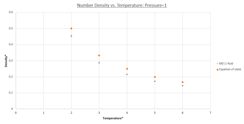  figure 15;Density vs. temperature, pressure = 1.0

• 
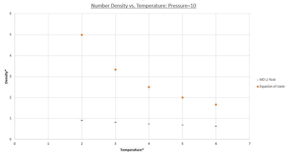  figure 16;Density vs. temperature, pressure = 10

To discuss the deviations seen in the above plots an understanding of the ideal gas law, its assumptions and when these are met by a system is required. An ideal gas assumption of a system is most appropriate when the system is both dilute and contains inert particles i.e ones that do not interact and are invisible to one-another. For example a dilute inert gas sample would be an ideal case. In these systems the total internal energy is wholly contributed to by individual particles kinetic energy, and the potential energy of the system is zero. In contrast the simulations utilize pairwise Lennard-Jones potentials and as such the PE contribution to the systems internal energy is non-zero. As a result both attractive and repulsive PE terms must be considered meaning the closeness of atoms inter-nuclear distances are limited by these factors, this is not the case for an ideal has.

For both pressure; 1.0 and 10, the deviation from the equation of state decreases with temperature, this can be understood by considering that each individual particles kinetic energy increases, given by the Maxwell-Boltzmann distribution and the equipartition principle. The systems behavior therefore tends toward that of an ideal gas system as the KE becomes dominant over the PE, given by pair-wise LJ potentials repulsive terms. Overall increased thermal motion causes both systems densities to decrease and a convergence seems to be occurring for the calculated values of system density.

It is seen that densities calculated using simulations at higher pressure deviate to a greater extent from the equation of state. This is because atoms are forced closer together on average increasing the overall potential energy of the system due to increased repulsive interactions causing the PE contribution of the system to dominate. As discussed before this is non-ideal behavior. In contrast atoms in an ideal gas system are easily pushed closer together due to a total lack of potential interactions meaning deviation in the density is far higher in the p=10 case than p=1 case.

JC: Good explanation of the trends with temperature and pressure.

Calculating the Heat Capacity using Statistical Physics

Heat capacity as described by statistical mechanics is different from other thermodynamic properties in that it is not an ensemble average but a measure of fluctuations about a systems internal energy equilibirum value. If one can determine the size of these fluctuations, of which are Gaussian with a standard deviation: $\sigma \widetilde{=}\frac{1}{\sqrt{N}}$ then the heat capacity can be calculated.

The definition of the heat capacity at constant volume in the [N, V, T] ensemble is as follows:

$C_V=\frac{\mathrm{V}\mathrm{a}\mathrm{r}\left[E\right]}{k_B{T}^2}=N^2\frac{⟨E^2⟩-{⟨E⟩}^2}{k_B{T}^2}$

The $N^2$ term is introduced in this definition as a correction factor due to the way LAMMPS calculates the heat capacity. The now calculated value will be extensive as it should be.

• The following two plots show the specific heat capacity per volume vs. temperature, once again the conditions (temperature and densities) chosen correspond to a Lennard-Jones super-critical fluid.
• The temperatures chosen: T₁ = 2, T₂ = 2.2, T₃ = 2.4, T₄ = 2.6, T₅ = 2.8
• The densities chosen: ρ₁ = 0.2 and ρ₂ = 0.8
• The time-step chosen: Δt = 0.0025 for the reason specified in the previous sections

• 
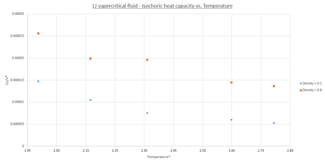  figure 17; Heat capacity per unit volume vs. temperature. Density:0.2 and 0.8

To discuss the trends shown it must be known simply that the heat capacity is also a measure of how easy a systems atoms are to excite thermally. Furthermore it is also defined as the amount of energy needed to raise the temperature of a system by one degree. Generally this means that heat capacity increases with temperature. However it is found that for supercritical Lennard-Jones fluids a decreasing linear trend, and a maxima are expected in the heat capacity of the system, the second of which occurs at the critical temperature itself. This trend is seen at both densities. The difference between densities of 0.2 and 0.8 is as expected for an extensive property like heat capacity as a higher density requires a smaller volume and as such there are a greater number of particles per volume which is why the plot for ρ = 0.8 is systematically higher but follows the same trend as at ρ = 0.2.

The linear decrease is hard to explain but is plausible a supercritical LJ-fluids energy level structure is analgous to that of the hydrogen atom in that the energy spacing between levels decreases as the energy of the states increase. Because of this the density of these electronic states increases. Remembering that the MD simulations are done in the classical regime in a temperature range of 240-360K. Therefore all the DoF of the system are all accessible, unlike for a H-atom, and the energy levels form a continuum band structure. To conclude as the the thermal energy available to the system increases higher energy states are accessible. As the density of states is greater at these energies the promotion energy needed to enter an unpopulated state and distribute this population in a thermal equilibrium is reduced and hence so is the heat capacity.

The temperature range modelled is shown in the graph below the same behaviour of the heat capacity is observed after the phase-transition to a LJ supercritical fluid.

• 
  figure 18; Lennard-Jones fluid critical heat capacity trend and maximum point[2]

JC: Brilliant analysis, well backed up by additional literature research, well done.

The input script used in LAMMPS is shown below:

### DEFINE SIMULATION BOX GEOMETRY ###
variable density equal 0.2
lattice sc ${density}
region box block 0 15 0 15 0 15
create_box 1 box
create_atoms 1 box

### DEFINE PHYSICAL PROPERTIES OF ATOMS ###
mass 1 1.0
pair_style lj/cut/opt 3.0
pair_coeff 1 1 1.0 1.0
neighbor 2.0 bin

### SPECIFY THE REQUIRED THERMODYNAMIC STATE ###
variable T equal 2.0
variable timestep equal 0.0025

### ASSIGN ATOMIC VELOCITIES ###
velocity all create ${T} 12345 dist gaussian rot yes mom yes

### SPECIFY ENSEMBLE ###
timestep ${timestep}
fix nve all nve

### THERMODYNAMIC OUTPUT CONTROL ###
thermo_style custom time etotal temp press
thermo 10

### RECORD TRAJECTORY ###
dump traj all custom 1000 output-1 id x y z

### SPECIFY TIMESTEP ###

### RUN SIMULATION TO MELT CRYSTAL ###
run 10000
unfix nve
reset_timestep 0

### BRING SYSTEM TO REQUIRED STATE ###
variable tdamp equal ${timestep}*100
fix nvt all nvt temp ${T} ${T} ${tdamp}
run 10000
reset_timestep 0

### MEASURE SYSTEM STATE ###
unfix nvt
fix nve all nve
thermo_style custom step etotal temp press density
variable etotal equal etotal
variable etotal2 equal etotal*etotal
variable temp equal temp
fix aves all ave/time 100 1000 100000 v_temp v_etotal v_etotal2 
run 100000

variable avetemp equal f_aves[1]
variable aveenergy equal f_aves[2]
variable aveenergy2 equal f_aves[3]
variable heat_capacity equal (((atoms)^2)*(f_aves[3]-(f_aves[2])^2))/(vol*((f_aves[1])^2))

print "heat_capacity ${heat_capacity}"
print "Temp ${avetemp}"

Structural properties and the Radial Distribution function

The radial distribution is an important statistical mechanical function as it captures the structure of liquids and amorphous solids. It is given by ρg(r) which yields the time-averaged radial density of particles at r with respect to a tagged particle at the origin. In this section the RDF of a Lennard-Jones vapour, liquid and solid is computed. Doing so requires system conditions that yield such phases, these are determined from a LJ phase diagram, avoiding the liquid-vapour coexistence and supercritical fluid regions.

• Vapour: ρ = 0.05, T = 1.2
• Liquid: ρ = 0.8, T = 1.3
• Solid: ρ = 1.2, T = 1.0

• 
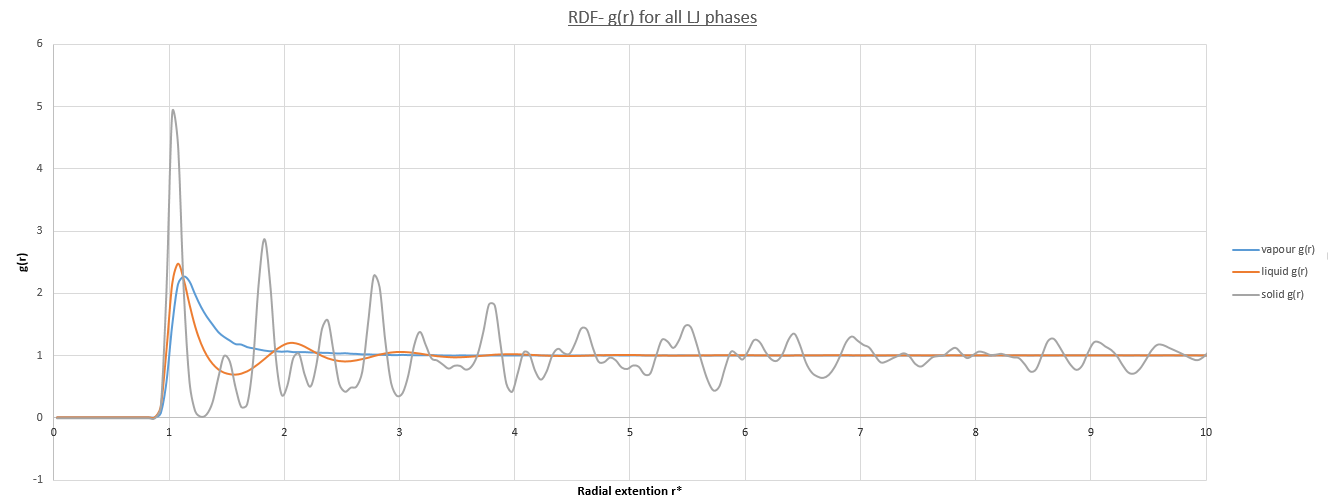  figure 20; RDF for all LJ phases vs. time, Δt=0.002 (pre-set)

It is key to note that all three phases only have a non-zero RDF at interatomic distances >0.9. Below this value corresponds to an excluded volume overlap and as such is highly unlikely to be occupied by a nieghbouring atom due to the very-strong LJ repulsive term, ∝r^-12,. Furthermore the time-step used <0.01 means that this phenomena will never occur. In addition, in all phases the RDF tends to/fluctuate about unity at large radial distances this is because particle distribution is totally uncorrelated as the LJ pair-wise potential tends to zero. There is no long-range structure present such that ρg(r) =1, which is simply the number of molecules per unit volume. Note that this value is normalized from 1.2 to 1.0. Each phase contains at least one peak in its RDF, the first of which are at very similar radial distances.

The liquid phase RDF contains three alternating peaks. The first and largest occurs at r_eq in the LJ potential minimum and nearest neighbours take advantage of this local PE well. The second peak occurs at a large radial distance and is a result of the nearest neighbouring atoms exclusion zone. These peaks alternate outwards resembling an expanding shell system of atomic packing. These peaks loose correlation with respect to the reference atom at the origin due to random thermal pertubations, which accumulate as the shells expand outward. The RDF has only 3 distinct peaks leading to the expected conclusion that the liquid phase has only short-range order up until an internuclear distance of approximately 4.0. It is seen that the local order is similar to that of the solid phase, but crucially this similarity decays rapidly with distance rendering a system with no-long order.

The vapour phase RDF on the other hand contains only one peak demonstrating this phase has even shorter-range order. This is also expected as the phase is much less dense and was simulated with a density of 0.05 compared to 0.8. It is energetically favorable due to larger system disorder and therefore entropy that just one nieghbouring atom exists before a return to the normalized system bulk density as any correlation beyond this would reduce the systems free energy.

The solid phase RDF has the most peaks of which occur over the entire course of the simulation. The major difference is the much sharper nature of these peaks when compared to the vapour and liquid phase RDF's. This is because the system is much more ordered, in fact the peaks refer to lattice points in an FCC lattice. To expand this picture at 0K where there is a total absence of thermal motion of atoms on their respective FCC lattice sites, the RDF would become a delta-function at exact lattice spacing's. However the peaks are not like this due to the non-zero temperature used in the simulation and hence decrease in amplitude due to Brownian motion similar to that discussed in the liquid phase. This effect is not as severe over the simulated radial distance due to the solids higher rigidity. However it is still possible to determine the lattice spacing's using the first three peaks in the solid RDF. Furthermore using the integral of the RDF as a function of radial distance yields the areas under each of these peaks. The magnitude of this area is equivalent to the number of atoms at that radial distance and therefore yields coordination numbers.

• 
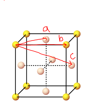  figure 21;Visualizing fcc lattice spacing's with reference to RDF peaks
• 
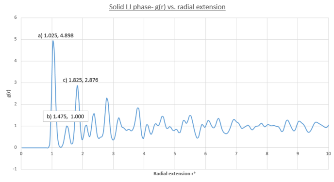  figure 22;Solid phase LJ- first three peaks

• 
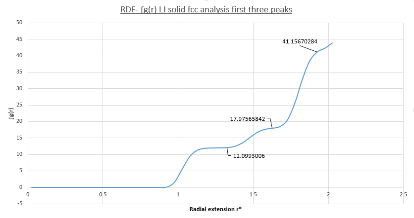  figure 23;RDF integral vs. radial extension cf. coordination numbers
• 
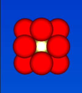  figure 24;FCC nearest-nieghbour coordination
• 
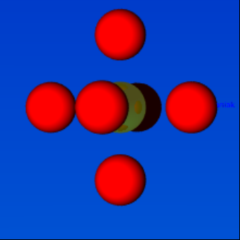  figure 25;FCC second nearest-nieghbour coordination
• 
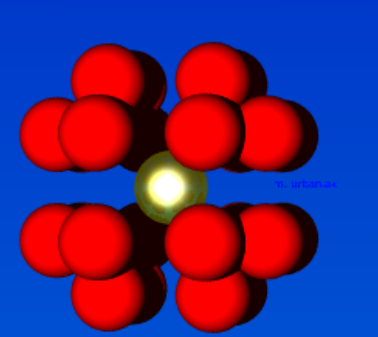  figure 26;FCC third nearest-nieghbour coordination

• It is therefore easy to see from the correspondence between figures 21 and 22 that the lattice spacing is equal to the radial distance from the RDF origin to the second peak: = 1.475

JC: Can you use the geometry of the unit cell to show whether the positions of the first and third peaks also agrees with this value for the lattice spacing?

• From figure 23 the isolated area corresponding to each peak in figure 22 is calculated and yields coordination numbers:

1. peak a) coordination number = 12-0 = 12- corresponds to figure 24 arrangement
2. peak b) coordination number = 18-12 = 6- corresponds to figure 25 arrangement
3. peak c) coordination number = 42-18 = 24- corresponds to figure 26 arrangement

To conclude the RDF in essence measures the effect Brownian motion due to the systems thermal energy has on the local and long range order of that system. Less dense phases such as the vapour phase have fewer pair-wise potential interactions, the sum of these determines an overall energy scale for the system. For the vapour phase as compared to the condensed phases this energy scale is of a lower relative magnitude compared to the thermal energy of the system. This means random thermal perturbations of the system have a larger effect. This leads to reduced long-range order and a faster return to bulk density RDF.

JC: Good, thorough explanation.

Dynamical Properties and the Diffusion Coefficient

Task 1- The Mean Squared Displacement (MSD)

The MSD of a system is a measure of the deviation of a particle with reference to its own time-averaged position. More specifically this deviation can be defined as the extent of spatial random motion explored by a random walker due to its Brownian motion due its inherent thermodynamic driving force to increase the systems overall entropy, and reduce its overall free energy. The result of such motion in systems is diffusion. The probability of finding a particle based of this motion with respect to its starting position can be described by a Gaussian distribution and hence the most likely position for it to be is it starting position. However the significance of the tails of such a distribution depend of the medium/phase the particle is in. Three regimes can occur depending on this which encapsulate the effect of different diffusive resistances, which are in fact the frequency of collisions with other particles in the system. These regimes can be quantified and visualized using the MSD plotted against values of the time-averaged timestep.

• Quadratic regime- A line curving upward with a quadratic relation to the time-step. Only pure diffusion of the particle is occurring i.e the trajectory of the particle is ballistic in nature. As a result each particles velocity is constant and therefore the distance travelled per time-step is also. The MSD is defined by the square of the variance, therefore in this regime MSD∝t².
• Linear regime- A completely straight line. This occurs when the particles trajectory is determined by Brownian motion as the frequency of collisions play an important role in the overall averaged deviation. This generally occurs in denser phases and to represent this MSD∝t.
• Plateau regime- MSD line plateaus as the time of simulation increases. This occurs when the particles motion is confined.

The MSD uses only one input data-set; the time-evolution of the particle- its trajectory and is defined by the following formula:

$\mathrm{M}\mathrm{S}\mathrm{D}\equiv ⟨(x-x_0{)}^2⟩=\frac{1}{T}\sum _{t=1}^T(x({\delta }_t)-x_0{)}^2$

This formula shows the averaged difference between to positions of a particle along the trajectory, separated by the simulation time-interval over the total simulation time frame T. Each of these averages is squared and the result is a description of the positional variance.

The MSD yields information regarding how far a particle deviates from its starting position in the simulation time-frame, the diffusivity constant of the system and what environment the particle is in.

The following plots show the MSD vs. Time-Averaged Timestep for the vapour, liquid and solid Lennard-Jones phases for both small system MD calculations conducted for this report (same conditions and timestep as before) and for a much larger system containing one-million atoms.

• Vapour MSD

• 
• 
• 
• 

JC: Fitting a straight line to the whole data set is a slightly misleading.

Two plots for both the small and large systems are shown. This is because the LJ vapour phase contains both a distinct quadratic regime and linear regime, the linear regime is needed to calculate the diffusion coefficient of the system. This system is the least dense of all those modelled and because of this until the 2000th timestep each particle does not encounter and collide a sufficient amount meaning trajectories are dominated by ballistic behaviour. However a transition to a linear regime occurs after this point because of attractive pair-wise Lennard-Jones potentials bringing particles closer together on average making collisions more frequent and Brownian behaviour starts to dominate. This transition can be quantified by the overall increase in R^{2} values, a statistical measure of linearity, from the entire simulation to that isolated after the 2000th timestep: 0.9869 to 0.9996 (small sim) and 0.9819 to 0.999 (1m sim).

• Liquid MSD

• 
• 

In contrast to the vapour phase MSD, the MSD for the liquid phase is entirely in the linear regime. This is expected due to the denser nature of the phase resulting in a far higher initial frequency of particle collisions and hence Brownian motion. This is quantified by the greater R^2 value over the entire simulation: 0.999. This does show the convergence of the vapour and liquid phase positional deviations at larger time-scales.

• Solid MSD

• 
• 

The solid phase MSD shows the biggest contrast in behaviour between all phases. The system is frozen and the MSD plateaus because kinetic energy pf the system is not sufficient enough to reach diffusive behavior. This plateau represents a finite MSD value inherent due to the solid LJ phases FCC-crystalline structure; atoms are held rigidly on unit cell lattice sites by very strong bonds, the energy scale of such a system far exceeds that of the systems thermal energy. As a result these atoms are confined to a limited radial distance from their respective lattice sites. This behaviour is quantified by the plots as the plateau value of the solid phase is far lower in magnitude, 0.0198, compared to the growing MSD values seen for the less dense phases. In addition the plots show a sharp spike up until the 87th time-step denoting the confined region atoms in the solid phase can explore. The extent of confinement of the particle is calculated by square-rooting the MSD plateau value as this will be characteristic of the confinement diameter in a Lennard-Jones FCC lattice - 0.128 (small sim) and 0.147 (1m sim), in reduced units.

JC: Again, good explanation of MSD behaviour.

Task 2- The Diffusion Coefficient (D)

The extent of the LJ systems diffusive behaviour in each of the phases can be contained in a single diffusive coefficient. This can be determined from the linear gradient of the MSD plots in the previous section because of its definition in 3D:

$D=\frac{1}{6}\frac{\partial ⟨r^2\left(t\right)⟩}{\partial t}$

The value of the diffusion coefficient was calculated for each phase for both the smaller D_Small and larger D_1M simulations by exploiting this relation with the MSD. For this calculation which ultilises the gradient of the MSD vs Timestep(t/Δt) plot and therefore values directly obtained will be in reduced units. These values still have the dimensionality commonly used for D, [L]²[T]^-1, but this needs to be converted into per unit time, not timestep, to yield the common S.I units [m²s^-1]. This is achieved by dividing all output values by the timestep, 0.0025.

• Vapour: D_Small = 1/6 * (0.0469/0.0025) = 3.127, D_1M = 2.413
• Liquid: D_Small = 0.093, D_1M = 0.068
• Solid: D_Small = 3.333x10^-7, D_1M = 3.333x10^-6

As expected from the MSD plots and diffusive behaviour of a less dense state, the diffusion coefficient for the vapour phase is far larger than either of the condensed phases. This is due to a lower collision frequency encountered along particle trajectories. Furthermore there is another striking decrease in values calculated when comparing the liquid and solid phases. As stated before this is because diffusive behaviour is essentially non-existent in the solid phase due to extremely high rigidity due to particles being fixed on their respective lattice sites.

Note that increasing the number of atoms simulated still leads to the same behaviour being simulated and identified in the phases. The only notable change is in the Gaussian nature of the MSD where there is a reduction in fluctuations in the solid state MSD due to a larger system size being simulated. This is quantified by the fact that a Gaussians FWHM can be calculated by the square root of the product of the diffusion coefficient and the total simulation time. The total simulation time for both sets of simulations was fixed at 5000 time-averaged time-steps therefore because the D-value calculated for the solid phase using one-million atoms is an order of magnitude larger the FWHM is reduced, and therefore the standard deviation/flucuations of the results is too.

Task 3- The Velocity Autocorrelation Function (VACF)

Autocorrelation functions are used in MD to determine time-dependent properties of atomic systems. The VACF does this by measuring the correlation of an atoms velocity after a certain number of time-steps with its own velocity at a previous time, in this report this is its initial equilibrium velocity as described by the Maxwell-Boltzmann relation. This is useful as it provides insight into the role inter-atomic forces, due to the Lennard-Jones potential, have on an atoms motion in time. It is defined mathematically as the following:

$C\left(\tau \right)=⟨\mathbf{v}\left(t\right)\cdot \mathbf{v}(t+\tau )⟩$

1D harmonic oscillator solution to the normalized VACF

The normalized VACF is given by the following equation:$C\left(\tau \right)=\frac{\underset{-\mathrm{\infty }}{\overset{\mathrm{\infty }}{\int }}v\left(t\right)v(t+\tau )\mathrm{d}t}{\underset{-\mathrm{\infty }}{\overset{\mathrm{\infty }}{\int }}{v}^2\left(t\right)\mathrm{d}t}$

Remembering the equation describing the 1D harmonic oscillators time-evolving position: $x(t)=Acos(\omega t+\varphi )$

Therefore the velocity for the system is given by the derivative: $v(t)=\frac{dx}{dt}=-A\omega sin(\omega t+\varphi )$

Squaring this yields: $v^2(t)=\frac{dx}{dt}=A^2{\omega }^{2}sin(\omega t+\varphi {)}^2$

Incorporating the timestep $\tau$ into the equation allows us to write out the normalized VACF as follows: $C(\tau )=\frac{\underset{-\mathrm{\infty }}{\overset{\mathrm{\infty }}{\int }}-A\omega sin(\omega t+\varphi )\times -A\omega sin(\omega (t+\tau )+\varphi )dt}{\underset{-\mathrm{\infty }}{\overset{\mathrm{\infty }}{\int }}{A}^2{\omega }^{2}sin(\omega t+\varphi {)}^{2}dt}$

The Amplitude and angular frequency terms outside the trigonometric functions cancel and we re-write the equation using the double angle formula for the sine terms in the numerator. It is key to couple the correct terms such that $sin(A+B)=sin((\omega t+\varphi )+\omega \tau )$ terms. This transformation and separating the numerator functions yields the following:

$C(\tau )=\frac{\underset{-\mathrm{\infty }}{\overset{\mathrm{\infty }}{\int }}cos(\omega t+\varphi )sin(\omega \tau )sin(\omega t+\varphi )dt}{\underset{-\mathrm{\infty }}{\overset{\mathrm{\infty }}{\int }}si{n}^2(\omega t+\varphi )dt}+\frac{\underset{-\mathrm{\infty }}{\overset{\mathrm{\infty }}{\int }}si{n}^2(\omega t+\varphi )cos(\omega \tau )dt}{\underset{-\mathrm{\infty }}{\overset{\mathrm{\infty }}{\int }}si{n}^2(\omega t+\varphi )dt}$

Now it is apparent why the couple of the correct terms was key. Because we are integrating with respect to time the isolated function $cos(\omega \tau )$ is a constant. It can therefore be removed from the second integral. This essential as it transforms the second improper integral such that it is now equal to unity. This is because the numerator and denominator integrands and limits are identical. Utilising the double angle formula for sin(2A) yields the following:

$C(\tau )=cos(\omega \tau )+sin(\omega \tau )\frac{1}{2}\times \frac{\underset{-\mathrm{\infty }}{\overset{\mathrm{\infty }}{\int }}(sin(\omega \tau )sin(2\omega t+2\varphi )dt}{\underset{-\mathrm{\infty }}{\overset{\mathrm{\infty }}{\int }}si{n}^2(\omega t+\varphi )dt}$

Now identifying the remaining numerator integrand as the product of two sine functions, and is therefore an odd function, integrating this between positive and negative values of the same arbitary limit, even if infinity, yields zero. Furthermore the denominator integrand is squared and as such can only take positive values. Integrating this between the limits of infinity yields infinity. In addition this could be showed by expanded using the double angle formula for cos(2A). In both cases an even function results. As a result the final fraction is equivalent to zero divided by infinity, therefore the second term equal zero.

This leaves the only remaining term $cos(\omega \tau )$ which is equal to $C(\tau )$ and is therefore the 1D harmonic oscillator solution to the normalized VACF.

JC: Maths is correct. The second use of the double angle formula is unnecessary as sin(x)cos(x) is already an odd function and so the integral from -infinity to infinity is zero.

Determining the Diffusion Coefficient using the VACF & Comparison 1D harmonic oscillator VACF with LJ liquid and solid

It is possible to use the VACF of a system as an alternative method to the MSD for calculating its diffusion coefficient. This is achieved by integrating the VACF over the simulation time frame:

$D=\frac{1}{3}\underset{0}{\overset{\mathrm{\infty }}{\int }}\mathrm{d}\tau ⟨\mathbf{v}\left(0\right)\cdot \mathbf{v}\left(\tau \right)⟩$

The following plots are again from MD simulations of a small system and of a larger system consisting of one-million atoms, however they are now plots of the running VACF integral vs. time-step. This was achieved by applying the trapezium rule to output data from LAMMPS and is useful as the diffusion coefficient can be calculated from the final summation.

• Vapour

• 
• 

• Liquid

• 
• 

• Solid

• 
• 

Values of the diffusion coefficient are calculated using final integral summation values seen on all plots. As before D_Small and D_1m denote values for the small and large atom number simulations. As for the MSD method for calculating D, the immediate values outputed are once again in reduced units. In contrast to the MSD calculation, the VACF method used the integral of a plot, VACF vs. Timestep and therefore the dimensionality of the D values is now [L]²([T]^-1/Δt) and therefore to obtain S.I units for D values, these outputs must be multiplied by the timestep, 0.0025.

• Vapour: D_Small = 1/3 * 4024.971086 * 0.0025 = 3.354, D_1M = 4.086
• Liquid: D_Small = 0.097, D_1M = 0.170
• Solid: D_Small = 1.554x10^-3, D_1M = 5.69x10^-5

These values follow the decreasing trend observed for the diffusion coefficients calculated using the MSD for each phase. The vapour system giving the largest value of D and the solid system having the smallest. Once again, the simulation using one-million atoms doesn't have any significant effect on the values on the magnitude of values for diffusion coefficients obtained. However it must be noted that a negative result was obtained for the solid D(small sim), using the VACF method. A negative diffusion coefficient would result from this value, which makes no physical sense. This error is due to the way the VACF is calculated as the sum of averaged product velocity at a time-origin and at a time, tau, later. At the end of the simulation the values of tau increase meaning the calculation can average over progressively fewer time-origins. For example: tau=3000, the calculation can use time origins at 0, 1, 2....3000, but for tau=6000 the calculation only has the time-origin at 0 available. To conclude the calculation of the VACF becomes more error prone at larger tau values. This error propagates into the integral VACF vs. timestep plots and results in the negative value in the case of the solid LJ phase. However this error is small it is seen that the integral does tend to zero as expected and the resulting D value is close to zero.

JC: Good understanding of the calculation of the VACF.

In terms of error, it is evident it was not too large as the discrepancies between the MSD and VACF method values of the calculated the diffusion coefficient are small. The most significant source of error can be assigned to the use of the trapezium rule for approximating the area under the VACF curves used to plot the running integrals and subsequently D. This method due to the geometry of a trapeziod always over-estimates the integral as the majority of the integrand in all cases are concave-up. This would not be the case if used for the periodic VACF of the 1D harmonic oscillator as both the concave-up over-estimations and concave-down under-estimations cancel when summed. To reduce this error a larger number of smaller trapezium can be used, however this is computationally expensive. Other methods of numerical integration of which have more accuracy for Gaussian distributed functions such as Gaussian quadrature could be used.

Furthermore the theory underlying the relationship between the VACF area and the diffusion coefficient only holds when the integral VACF of the system decays to zero in the simulation time. For the solid system, the assumption that this condition is met is arguable and therefore error will be introduced into the D value calculated for this system and could also have been the cause of the negative D obtained for the solid LJ phase. Evidence for this can be drawn from the discrepancies in D-values calculated for the different LJ phases for the small and large atom count simulations. Furthermore the way the VACF is orginally calculated leads to increasing errors as the simulation progresses and could also be a cause of the negative D value for the solid LJ phase. A clear anomaly can be seen between the MD calculations conducted for this report and the larger simulations only for the solid phase. The one-million atom system where the VACF did decay to zero with a high degree of accuracy calculated a D value of at least entire order of magnitude larger. This lack of convergence also manifested itself in a large difference in the MSD calculations of D. Finally, absolute error could be reduced by simply simulating more precise particle trajectories, however this would require a smaller timestep and therefore would also be more computationally expensive due to reasons discussed previously.

Referring back to the definition of the VACF it is seen that it utilises a summation of the scalar product of a velocity after a certain number of timesteps and an initial starting velocity for all atoms in a system. Because all systems modelled are entirely classical, Newton's laws state that for an atom with a specific velocity that undegoes no collisions (i.e it is isolated) will retain this velocity for the simulation/all time and the VACF would be a horizontal line equal to one (normalized). However a system where inter-atomic forces are weak, but not negligible, Newton's same laws state the magnitude and/or direction of a particles velocity will change gradually. In other words the systems overall velocity will decorrelate in time but only due to diffusive behaviour, this is seen for non-dense systems such as the LJ vapour pahse where this decay in correlation is exponential in form, this is shown below:

• 

The following plot displays the VACF's for the 1D harmonic oscillator found in the previous section on the same axes as the solid and liquid LJ VACF's. This is plotted for timesteps between 0 and 500.

• 

[Note that initial values of the solid and liquid LJ VACF's are not normalized and should be equal to one for obvious reasons.]

The harmonic oscillator simulated was a single isolated oscillator it therefore never collides with other particles and as such its time-evolving velocity never de-synchronizes. As stated before, the VACF is defined vectorially in such a way that for a single oscillator the dot product of velocities at different time-steps equal negative one when a particle is traveling with the same speed but in the opposite direction and vice-versa for a value of one. Additionally the value of zero corresponds to the harmonic oscillator in a state with maximum potential energy and therefore no kinetic energy. This behaviour is periodic as correlation is over time is never lost due to a total absence of collisions and explains the harmonic oscillator solution to the normalized VACF.

Contrary to the discussion for the non-dense LJ vapour phase, atoms in denser phases such as the solid and liquid phases encounter far stronger inter-atomic forces. Atoms in these systems observe significant order as discussed in the RDF section this is because atoms seek out internuclear distance arrangements in the LJ potential minima and away from excluded volumes for energetic stability. In solids strong internuclear forces cause these ordered locations to become very stable resulting in a lattice structure, and the atoms cannot escape easily from their lattice points.

Atomic motion in a solid LJ VACF should therefore appear similar as each atom's motion - vibrating and relaxing about its lattice point can be modelled as a simple harmonic oscillator, this is seen as the VACF function function oscillates strongly from positive to negative values. This is a reasonable assumption because as just discussed the atoms are confined to vibrate in a small radius about their lattice points and affords for an easy comparison to the isolated harmonic oscillators behaviour. However a large difference occurs in these two systems VACF's because the VACF is an average over all of these small oscillators and because each is not isolated collisions occur that disrupt the perfect oscillatory motions. De-synchronization therefore starts to dominate due to these pertubative collisions after 50 timesteps causing the overall distribution of velocities to become randomized. This results in a VACF resembling damped harmonic motion and hence there is a total VACF of zero after a finite period of time. It should be noted that before this correlation similar to the harmonic oscillator was observed as a single distinct peak at 38 timesteps. To conclude the LJ solid VACT depicts a system that behaves more like a point as compared to the isolated harmonic oscillator after the duration of the simulation.

Both the solid and liquid VACF's observe this behaviour as the liquid also showed fleeting oscillatory behaviour, manifesting itself in a single peak occurring at around 65 timesteps. Recalling findings from the RDF's of both the solid and liquid states; a liquids local order is very similar to that of a solid as similar RDF peaks occured due to a local atomic shell system. However the liquid RDF decayed very quickly as a the liquid observed no long-range order due to a lower density and weaker interatomic interactions on average. This single peak can be understood as in this phase atoms do not have fixed regular "lattice" positions. Refering back to the magnitude of diffusion coefficients calculated for the liquid and solid LJ phases, the liquid phase D-value are at least five orders of magnitude greater than for the solid phase for both the MSD and VACF methods. Therefore diffusive motion of the system contributes far more to the rapidly decaying oscillatory motion seen in the liquid VACF. The single peak can be described as one very damped oscillation before complete de-correlation occurs, this may be considered a collision between two atoms before they rebound from one another and diffuse away.

JC: Great, very thorough analysis.

Conclusion

Using a simple Lennard Jones pair-wise potential system, this report has demonstrated the stark differences in structure and behaviour of the solid, liquid and vapour phases. This is summarised particularly well in 'Soft Condensed Matter, R.A. Jones, Oxford 2002.' where Jones makes clear the relative effects different levels of thermal perturbation have on the physical state of a system. I will use his concise summary alongside computational evidence found throughout this report to explain these differences more roundly.

In the vapour phase at high temperatures molecules are in a state of constant motion where the attractive forces, dictated by the LJ potential in this report, are weak compared to the thermal energy. These molecules infrequently collide such that there is very little correlation between the motions of individuals. This was evidenced in the VACF, dictated purely by diffusion and a ballistic trajectory and was seen as short time scales of the simulation. In this state the system approximates fairly well with the familiar ideal gas, seen in the convergence of the simulated systems densities with the equation of state as the temperature was increased in section 3.4. As the temperature is reduced, attractive interactions that occur during collisions start to become more significant. The relative motions between individuals particles start to become correlated and the system tends to more dense state where collisions are frequent, which is characterised by the vapour VACF transition to the linear regime. The total system energy is still kinetically dominated, however the energies of interactions in the transient clusters start to become significant and we head towards a phase transition. This transition occurs when these correlations become permanent and substantial short-range order starts to occur, characteristic of the denser liquid phase.

The attractive and repulsive terms of this interactive Lennard-Jones potential both play a significant role in this new ordering. There is a balance between the tension of the attractive and repulsive terms, mathematically given by their respective r^-6 and r^-12 power laws. The attractive term tries to pack molecules as closely as possible- as seen to be in the LJ -ε potential well - and the repulsive term which imposed a minimum separation characteristic of an exclusion volume. This ordering was seen in the RDF plots of the liquid phase where oscillating probability densities for nieghbouring particles was seen to be at finite radial distances characterised by a short-range atomic shell system producing only one distinct peak. As the temperature/system perturbation decreases further it becomes favorable to pack molecules in a regular rather than random way, achieving a higher density of molecules whilst still satisfying a minimum distance constraint. Here the system has entered the solid phase and such a system was identified by its RDF to demonstrate significant long-range order characteristic of an FCC crystal lattice. The area under each curve and lattice separation was calculated yielding useful information concerning the crystal structure and coordination spheres. The VACF of these phases was compared to that of an isolated harmonic oscillator and it was still found that thermal perturbations de-synchronized molecular motion, though less rapidly, but the overall order of the system is far less perturbed, leading to the permanent ordering of particles.