Talk:Mod:Tfy286

JC: General comments: Most tasks attempted, but some of the written explanations lacked a bit of detail. Make sure you have a good understanding of the theoretical background to the tasks and use this to explain the trends that you see in your results.

Introduction to molecular dynamics simulation

Task

1. 1). Open the file HO.xls. In it, the velocity-Verlet algorithm is used to model the behaviour of a classical harmonic oscillator. Complete the three columns "ANALYTICAL", "ERROR", and "ENERGY": "ANALYTICAL" should contain the value of the classical solution for the position at time $t$, "ERROR" should contain the absolute difference between "ANALYTICAL" and the velocity-Verlet solution (i.e. ERROR should always be positive -- make sure you leave the half step rows blank!), and "ENERGY" should contain the total energy of the oscillator for the velocity-Verlet solution. Remember that the position of a classical harmonic oscillator is given by $x\left(t\right)=A\cos (\omega t+\varphi )$ (the values of $A$, $\omega$, and $\varphi$ are worked out for you in the sheet).

2). For the default timestep value, 0.1, estimate the positions of the maxima in the ERROR column as a function of time. Make a plot showing these values as a function of time, and fit an appropriate function to the data.

2. Experiment with different values of the timestep. What sort of a timestep do you need to use to ensure that the total energy does not change by more than 1% over the course of your "simulation"? Why do you think it is important to monitor the total energy of a physical system when modelling its behaviour numerically?

The maximum energy is 0.5. If the total energy does not change by more than 1%, the minimum energy should be 0.5*(1-1%)=0.495. Therefor the timestep is required to change to 0.2 (or less than 0.2). Here is the new diagram when timestep equals to 0.2.

JC: What is the equation for the straight line that you've plotted through the maxima in the error? Why does the error oscillate over time? Good choice of timestep.

3. For a single Lennard-Jones interaction, $\varphi \left(r\right)=4ϵ(\frac{{\sigma }^{12}}{r^{12}}-\frac{{\sigma }^6}{r^6})$, find the separation, $r_0$, at which the potential energy is zero. What is the force at this separation? Find the equilibrium separation, $r_{eq}$, and work out the well depth ($\varphi \left(r_{eq}\right)$). Evaluate the integrals $\underset{2\sigma }{\overset{\mathrm{\infty }}{\int }}\varphi \left(r\right)\mathrm{d}r$, $\underset{2.5\sigma }{\overset{\mathrm{\infty }}{\int }}\varphi \left(r\right)\mathrm{d}r$, and $\underset{3\sigma }{\overset{\mathrm{\infty }}{\int }}\varphi \left(r\right)\mathrm{d}r$ when $\sigma =ϵ=1.0$.

1). when potential energy=0,

$(\frac{{\sigma }^{12}}{r^{12}}-\frac{{\sigma }^6}{r^6})$=0. So,$r_0$= $\sigma$.

2). energy is zero, so net force is zero as well.

JC: The force is the first derivative of the potential, so it is not necessarily zero when the energy is zero, look at a plot of the Lennard-Jones potential, when the potential is zero is the gradient also zero?

3). at $r_{eq}$, potential energy is minimum, $\frac{d\varphi }{dr}$ = 0,

$\frac{48ϵ{\sigma }^{12}}{{\sigma }^{13}}$ = $\frac{24ϵ{\sigma }^6}{{\sigma }^7}$

So, $r_{eq}$ = $\sqrt{2}\sigma$

JC: At r_eq, r is not sigma, the correct answer should be r = 2^(1/6)*sigma.

4). $\underset{2\sigma }{\overset{\mathrm{\infty }}{\int }}\varphi \left(r\right)\mathrm{d}r$= $\frac{-4r^{-11}}{11}+\frac{4r^{-5}}{5}=-0.0248$

$\underset{2.5\sigma }{\overset{\mathrm{\infty }}{\int }}\varphi \left(r\right)\mathrm{d}r$=$-8.177*10^{-3}$

$\underset{3\sigma }{\overset{\mathrm{\infty }}{\int }}\varphi \left(r\right)\mathrm{d}r$=$-3.29*10^{-3}$

JC: Correct.

4. Estimate the number of water molecules in 1ml of water under standard conditions. Estimate the volume of 10000 water molecules under standard conditions.

1). density of water is $1g/c{m}^3$, no.(water)= $\frac{1}{18}*6.023*10^{23}$= $3.346*10^{22}$

2). $\frac{1}{3.346*10^{22}}$=$\frac{volume(H2O)}{10000}$, so volume of 10000 water molecules is $2.98*10^{-19}$

5. Consider an atom at position $(0.5,0.5,0.5)$ in a cubic simulation box which runs from $(0,0,0)$ to $(1,1,1)$. In a single timestep, it moves along the vector $(0.7,0.6,0.2)$. At what point does it end up, after the periodic boundary conditions have been applied?

The new position $(0.5+0.7,0.5+0.6,0.5+0.2)=(1.2,1.1,0.7)$.

However it follows the periodic boundary condition, so it should be $(0.2,0.1,0.7)$.

6.The Lennard-Jones parameters for argon are $$\begin{gathered} \sigma =0.34\mathrm{n}\mathrm{m},ϵ \\ / \\ {k}_B=120\mathrm{K} \end{gathered}$$. If the LJ cutoff is $r^{*}=3.2$, what is it in real units? What is the well depth in $$\begin{gathered} {\mathrm{k}\mathrm{J} \\ \mathrm{m}\mathrm{o}\mathrm{l}}^{-1} \end{gathered}$$? What is the reduced temperature $T^{*}=1.5$ in real units?

1) r= 0.34* 3.2 nm = 1.088nm

2) $$\begin{gathered} ϵ \\ / \\ {k}_B=120\mathrm{K} \end{gathered}$$

$ϵ=120*1.38*10^{-23}*10^{-3}*6.023*10^{23}kJ/mol=0.9974kJ/mol$

3) T= 120* 1.5 K = 180K

JC: Correct.

Equilibration

task

1. Why do you think giving atoms random starting coordinates causes problems in simulations? Hint: what happens if two atoms happen to be generated close together?

If two atoms are too close together, there will be a huge repulsion existing between them. In order to calculate the huge energy change, the timestep should be very small. Therefore the computation process will be much more difficult.

JC: Good, the simulation will crash unless a much smaller timestep is used.

2. Satisfy yourself that this lattice spacing corresponds to a number density of lattice points of 0.8. Consider instead a face-centred cubic lattice with a lattice point number density of 1.2. What is the side length of the cubic unit cell?

there are four lattice points per volume per unit cell in a face-centred cubic.

$\sqrt[3]{\frac{4}{1.2}}=1.4938$

3. Consider again the face-centred cubic lattice from the previous task. How many atoms would be created by the create_atoms command if you had defined that lattice instead?

4*(10*10*10) = 4000 atoms will be created.

JC: Correct.

4. Using the LAMMPS manual, find the purpose of the following commands in the input script:

mass 1 1.0:

1 indicates the atom type, here is type 1.

1.0 indicates the atom mass, here is 1.0

pair_style lj/cut 3.0:

pair_style lj/cut means cutoff Lennard-Jones potential with no Coulomb,

3.0 is the arguments used by a particular style

pair_coeff * * 1.0 1.0:

asterisks here are used in place of or in conjunction with the I,J arguments to set the coefficients for multiple pairs of atom types.

1.0 and 1.0 here are the coefficients for the atom types

JC: What are the force field coefficients for the Lennard-Jones potential? Why is a cutoff used with this potential?

5. Given that we are specifying \mathbf{x}_i\left(0\right) and \mathbf{v}_i\left(0\right), which integration algorithm are we going to use?

velocity-Verlet algorithm

6. Look at the lines below.

### SPECIFY TIMESTEP ###
variable timestep equal 0.001
variable n_steps equal floor(100/${timestep})
variable n_steps equal floor(100/0.001)
timestep ${timestep}
timestep 0.001

### RUN SIMULATION ###
run ${n_steps}
run 100000

The second line (starting "variable timestep...") tells LAMMPS that if it encounters the text ${timestep} on a subsequent line, it should replace it by the value given. In this case, the value ${timestep} is always replaced by 0.001. In light of this, what do you think the purpose of these lines is? Why not just write:

timestep 0.001
run 100000

If the timestep is fixed at 0.001, once the timestep is required to change, all the timesteps will change into other values by hand.

However, if the timestep is set as a variable, only the first line is required to change, and the rest of them will change automatically.

JC: Correct.

7.1) make plots of the energy, temperature, and pressure, against time for the 0.001 timestep experiment (attach a picture to your report).

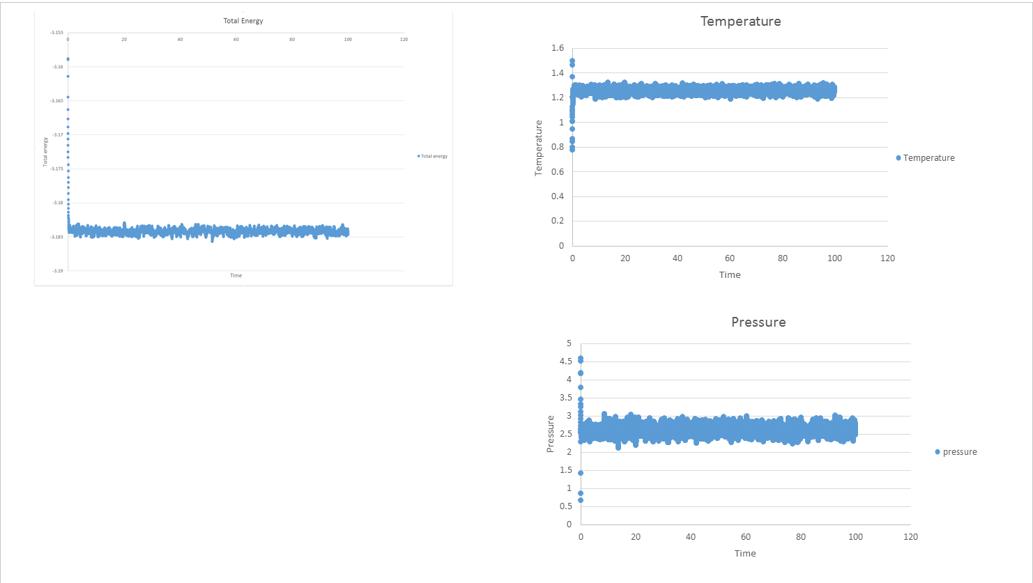
2) Does the simulation reach equilibrium? How long does this take?

Yes, the simulation reaches equilibrium when time= 0.43

3) make a single plot which shows the energy versus time for all of the timesteps (again, attach a picture to your report).

4)Choosing a timestep is a balancing act: the shorter the timestep, the more accurately the results of your simulation will reflect the physical reality; short timesteps, however, mean that the same number of simulation steps cover a shorter amount of actual time, and this is very unhelpful if the process you want to study requires observation over a long time. Of the five timesteps that you used, which is the largest to give acceptable results? Which one of the five is a particularly bad choice? Why?

0.01 is the largest to give acceptable result. And 0.015 is a particular bad choice because there is a big deviation from the others.

JC: Make the x axis range equal to the length of the shortest simulation. Should the average total energy depend on the choice of timestep? 0.0025 is the best choice as it gives the same results as shorter timesteps (0.001), but simulations can cover a larger length of time.

Running simulations under specific conditions

Task

1. Choose 5 temperatures (above the critical temperature T^* = 1.5), and two pressures (you can get a good idea of what a reasonable pressure is in Lennard-Jones units by looking at the average pressure of your simulations from the last section). This gives ten phase points — five temperatures at each pressure. Create 10 copies of npt.in, and modify each to run a simulation at one of your chosen \left(p, T\right) points. You should be able to use the results of the previous section to choose a timestep. Submit these ten jobs to the HPC portal. While you wait for them to finish, you should read the next section.

Pressure	Temperature
2.7 , 2.8	1.8 , 1.9 , 2.0 , 2.1 , 2.2

2. We need to choose $\gamma$ so that the temperature is correct $T=\mathfrak{𝔗}$ if we multiply every velocity $\gamma$. We can write two equations:

$\frac{1}{2}\sum _i{m}_i{v}_i^2=\frac{3}{2}N{k}_{B}T$

$\frac{1}{2}\sum _i{m}_i{\left(\gamma v_i\right)}^2=\frac{3}{2}N{k}_B\mathfrak{𝔗}$. Solve these to determine $\gamma$.

So, $\sum _i{m}_i{\left(\gamma v_i\right)}^2=3N{k}_B\mathfrak{𝔗}$

$\gamma =\frac{1}{\sum _i{v}_i}\sqrt{\frac{3N{k}_B}{\sum _i{m}_i}}$

JC: Not quite, take gamma out of the sum and then substitute the sum for the equation involving the current temperature, T, to get $\gamma =\frac{\mathfrak{𝔗}}{T}$.

3. Use the manual page to find out the importance of the three numbers 100 1000 100000. How often will values of the temperature, etc., be sampled for the average? How many measurements contribute to the average? Looking to the following line, how much time will you simulate?

100 stands for the number of input values every this many timesteps

1000 stands for the number of times to use input values for calculating averages

100000 stands for calculate averages every this many timesteps

Therefore the value of temperature will sampled for 1000 times. And there are 1000 measurements contributing to the average.

JC: Add more detail to show that you understand what the manual is saying about these three values.

4. 1). When your simulations have finished, download the log files as before. At the end of the log file, LAMMPS will output the values and errors for the pressure, temperature, and density $\left(\frac{N}{V}\right)$. Use software of your choice to plot the density as a function of temperature for both of the pressures that you simulated. Your graph(s) should include error bars in both the x and y directions. Does the discrepancy increase or decrease with pressure?

The higher the pressure the discrepancy increases.

2). You should also include a line corresponding to the density predicted by the ideal gas law at that pressure. Is your simulated density lower or higher? Justify this.

according to the ideal gas law, $pV=N{k}_{B}T$

$density=\frac{N}{V}=\frac{p}{k_{B}T}=\frac{p}{T}$, $k_B=1$(reduced unit)

The simulated density is lower than the ideal density. Because there are interaction forces existing among particles. When the pressure is applied, the repulsion between particles becomes dominant, and the distance between particles will be larger, so the density will be lower than the ideal situation.

JC: Show all results on the same axes so that the trend with pressure is clear and don't plot a straight line between data points, especially for the ideal gas as the ideal gas law doesn't follow this trend (density is proportional to 1/T). How does the discrepancy change with temperature?

Calculating heat capacities using statistical physics

Task

1. input script

### DEFINE PARAMETERS ###
variable D equal 0.2
variable T equal 2.8
variable timestep equal 0.0075

### DEFINE SIMULATION BOX GEOMETRY ###
lattice sc ${D} 
region box block 0 15 0 15 0 15
create_box 1 box
create_atoms 1 box

### DEFINE PHYSICAL PROPERTIES OF ATOMS ###
mass 1 1.0
pair_style lj/cut/opt 3.0
pair_coeff 1 1 1.0 1.0
neighbor 2.0 bin

### ASSIGN ATOMIC VELOCITIES ###
velocity all create ${T} 12345 dist gaussian rot yes mom yes

### SPECIFY ENSEMBLE ###
timestep ${timestep}
fix nve all nve

### THERMODYNAMIC OUTPUT CONTROL ###
thermo_style custom time etotal temp press
thermo 10

### RECORD TRAJECTORY ###
dump traj all custom 1000 output-1 id x y z

### SPECIFY TIMESTEP ###

### RUN SIMULATION TO MELT CRYSTAL ###
run 10000
unfix nve 
reset_timestep 0

### BRING SYSTEM TO REQUIRED STATE ###
variable tdamp equal ${timestep}*100
fix nvt all nvt temp ${T} ${T} ${tdamp} 
run 10000
reset_timestep 0
unfix nvt
fix nve all nve

### MEASURE SYSTEM STATE ###
thermo_style custom step etotal temp press density atoms
variable dens equal density
variable dens2 equal density*density
variable temp equal temp
variable temp2 equal temp*temp
variable press equal press
variable press2 equal press*press
variable atomss equal atoms
variable etotal equal etotal
variable etotal2 equal etotal*etotal


fix aves all ave/time 100 1000 100000 v_dens v_temp v_press v_dens2 v_temp2 v_press2 v_etotal v_etotal2
run 100000

variable avedens equal f_aves[1]
variable avetemp equal f_aves[2]
variable avepress equal f_aves[3]
variable errdens equal sqrt(f_aves[4]-f_aves[1]*f_aves[1])
variable errtemp equal sqrt(f_aves[5]-f_aves[2]*f_aves[2])
variable errpress equal sqrt(f_aves[6]-f_aves[3]*f_aves[3])
variable energyvariance equal (f_aves[8]-f_aves[7]*f_aves[7])
variable heatcap equal ${atomss}*${avedens}*${energyvariance}/(f_aves[5])
print "Averages"
print "--------"
print "Density: ${avedens}"
print "Stderr: ${errdens}"
print "Temperature: ${avetemp}"
print "Stderr: ${errtemp}"
print "Pressure: ${avepress}"
print "Stderr: ${errpress}"
print "heatcap per volume: ${heatcap}"

2. Plot C_V/V as a function of temperature

JC: How does the heat capacity change with density? Can you give any suggestions about why the heat capacity decreases with temperature?

Structural properties and the radial distribution function

Task

1. perform simulations of the Lennard-Jones system in the three phases. When each is complete, download the trajectory and calculate g(r) and $\int g(r)\mathrm{d}r$. Plot the RDFs for the three systems on the same axes, and attach a copy to your report.

2. Discuss qualitatively the differences between the three RDFs, and what this tells you about the structure of the system in each phase. In the solid case, illustrate which lattice sites the first three peaks correspond to. What is the lattice spacing? What is the coordination number for each of the first three peaks?

g(r) shows several peaks in the liquid state, which means the probability at these radial distances will be much higher than the others. Secondly, there are much more peaks observed in solid phases. The peak differences are caused by the different interaction forces. In liquid phases, the attractive force is dominant, and in the solid phase, the structure is regular and periodic, the interaction is stronger than in liquid phase, and the repulsive force is dominant. For face centred cubic, regarding (0,0,0) as a center, the first three peaks correspond to (1/2,1/2,0), (1,0,0) and (1,1,0). The difference from 0 to the second peak is the lattice point, 1.475.

JC: The solid has peaks at large r which indicates long range order, the liquid only has short range order. A diagram of an fcc lattice to show the atoms responsible for the first 3 peaks would have been good, did you calculate the coordination numbers as well - you can get these from the integral if you zoom in to look at the r values of the first 3 peaks. Could you have calculated the lattice parameter from the first and third peaks as well and taken an average, how does it compare with the initial value that you use in the LAMMPS script?

Dynamical properties and the diffusion coefficienT

Task

1. make a plot for each of your simulations (solid, liquid, and gas), showing the mean squared displacement (the "total" MSD) as a function of timestep. Are these as you would expect? Estimate D in each case. Be careful with the units! Repeat this procedure for the MSD data that you were given from the one million atom simulations.

MSD(SOLID)	MSD(LIQUID)	MSD(GAS)

JC: Are these plots for your simulation data or the data that you are given. Is the solid MSD what you'd expect - it doesn't look like the atoms are confined to lattice sites, did you change the lattice type to fcc? Show the lines of best fit on the graphs.

Because $MSD=⟨(x(t)-x_0{)}^2⟩=2Dt$,

$D=\frac{MSD}{2t}$

For solid, D = 0.0273/(2*0.016991) = 0.803

For liquid, D = 2.81/(2*1.67448) = 0.839

For gas, D = 12.9/(2*7.74)= 0.8333

the MSD data given

JC: Can you explain these graphs, are the data for the three phases on top of each other, is this what you would expect?

$D=\frac{1}{3}\underset{0}{\overset{\mathrm{\infty }}{\int }}C\left(\tau \right)$

2. 1). In the theoretical section at the beginning, the equation for the evolution of the position of a 1D harmonic oscillator as a function of time was given. Using this, evaluate the normalised velocity autocorrelation function for a 1D harmonic oscillator (it is analytic!):

$C\left(\tau \right)=\frac{\underset{-\mathrm{\infty }}{\overset{\mathrm{\infty }}{\int }}v\left(t\right)v(t+\tau )\mathrm{d}t}{\underset{-\mathrm{\infty }}{\overset{\mathrm{\infty }}{\int }}{v}^2\left(t\right)\mathrm{d}t}$

Be sure to show your working in your writeup.

For a 1D harmonic oscillator

$x\left(t\right)=A\cos (\omega t+\varphi )$

Therefore

$v\left(t\right)=-A\omega \sin (\omega t+\varphi )$

and

$v(t+\tau )=-A\omega \sin (\omega (t+\tau )+\varphi )$

Because $C\left(\tau \right)=\frac{\underset{-\mathrm{\infty }}{\overset{\mathrm{\infty }}{\int }}v\left(t\right)v(t+\tau )\mathrm{d}t}{\underset{-\mathrm{\infty }}{\overset{\mathrm{\infty }}{\int }}{v}^2\left(t\right)\mathrm{d}t}$

For the upper integration:

$\underset{-\mathrm{\infty }}{\overset{\mathrm{\infty }}{\int }}v\left(t\right)v(t+\tau )dt$

$=A^2{\omega }^2\underset{-\mathrm{\infty }}{\overset{\mathrm{\infty }}{\int }}sin(\omega (t+\tau )+\varphi )sin(\omega t+\varphi )dt$

$=A^2{\omega }^2\underset{-\mathrm{\infty }}{\overset{\mathrm{\infty }}{\int }}sin(\omega t+\varphi )(sin(\omega t+\varphi )cos(\omega \tau )+sin(\omega \tau )cos(\omega t+\varphi ))dt$

$=A^2{\omega }^{2}cos(\omega \tau )\underset{-\mathrm{\infty }}{\overset{\mathrm{\infty }}{\int }}si{n}^2(\omega t+\varphi )dt+A^2{\omega }^{2}sin(\omega \tau )\underset{-\mathrm{\infty }}{\overset{\mathrm{\infty }}{\int }}sin(\omega t+\varphi )cos(\omega t+\varphi )dt$

For the lower integration:

$\underset{-\mathrm{\infty }}{\overset{\mathrm{\infty }}{\int }}{v}^2\left(t\right)dt$

$=A^2{\omega }^2\underset{-\mathrm{\infty }}{\overset{\mathrm{\infty }}{\int }}si{n}^2(\omega t+\varphi )dt$

So,

$C\left(\tau \right)=cos(\omega \tau )+sin(\omega \tau )\underset{-\mathrm{\infty }}{\overset{\mathrm{\infty }}{\int }}\frac{cos(\omega t+\varphi )}{sin(\omega t+\varphi )}$

$=cos(\omega \tau )+sin(\omega \tau )\frac{ln(|sin(\omega t+\varphi )|)}{\omega }$

from $-\mathrm{\infty }$ to $\mathrm{\infty }$,

$C\left(\tau \right)=cos(\omega \tau )$

JC: Correct result, but check your working again, you cannot simplify the integrals like you have done. You can make the derivation easier and avoid doing any integration by recognising the integrands as even and odd functions and simplifying them accordingly.

2). On the same graph, with x range 0 to 500, plot $C\left(\tau \right)$ with $\omega =1/2\pi$ and the VACFs from your liquid and solid simulations.

$C\left(\tau \right)=cos(\frac{1}{2}\pi \tau )+2\frac{sin(\frac{1}{2}\pi \tau )}{\pi }$

3). What do the minima in the VACFs for the liquid and solid system represent? Discuss the origin of the differences between the liquid and solid VACFs. The harmonic oscillator VACF is very different to the Lennard Jones solid and liquid. Why is this? Attach a copy of your plot to your writeup.

The minima represents the starting points of self-diffusion. The origin of the differences is the interaction force difference. The interaction is larger , so the diffusion coefficient is smaller, which can be also observed by the area difference under the VACF(r) curve of two different phases.

JC: Look at the equation for the VACF, when is it negative and so when do the minima occur? Collisions between particles randomise particle velocities and cause the VACF to decorrelate, there are not collisions in the harmonic oscillator so it doesn't decay. You should have plotted the harmonic oscillator VACF with omega = 1/(2*pi). Did you try to calculate the running integral of the VACF or the diffusion coefficient from this?