Talk:Mod:SUNG95

JC: General comments: Report shows a good understanding of the material and the underlying theory. Make sure that you show all of the parts of each task as a few of the tasks were incomplete.

Theory

The Velocity-Verlet Algorithm

x(t) derived from the velocity-Verlet algorithm compared with the position of the classical harmonic oscillator.

Total energy of the system with respect to time

The error derived by comparing the solution of the velocity-Verlet algorithm with the position of the classical harmonic oscillator

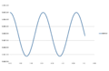
The three graphs above display the position of an atom, the total energy of the system and the error between the two methods of calculating the atom position.

Maximum Error against Time

From this graph of Maximum error vs Time, we can see that error increases with time at a stable linear rate.

---

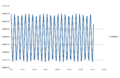
Running the same calculations with varying timesteps show the importance of choosing the right value of the timestep:

• 
  Energy at timestep=0.05
• 
  Energy at timestep=0.5
• 
  Error at timestep=0.5
• 
  Error at timestep=0.05

Examining the four additional graphs above, we can notice that a shorter timestep is able to provide a smaller value for error and that the energy fluctuates less than when a bigger value of timestep is used. However, a shorter timestep results in a shorter simulation type, which can result in a less realistic simulation. It is therefore important to find the right balance between the two.

Through trial and error, it has been found that timestep = 0.2850 or lower results in an energy fluctuation that is smaller than 1% over the course of the simulation. A small fluctuation in energy indicates higher resemblance to reality as technically the total energy should not fluctuate at all due to the Law of Conservation of Energy.

JC: Good choice of timestep. Why does the error fluctuate?

Lennard-Jones Potential

The equation to calculate the Lennard-Jones potential is as follows:

$\varphi \left(r\right)=4ϵ(\frac{{\sigma }^{12}}{r^{12}}-\frac{{\sigma }^6}{r^6})$

By equating this to 0, we find that the $r_0$, the separation at which the potential is 0, is $r_0=\sigma$.

We can then find the force at this separation by differentiating the Lennard-Jones potential with respect to r, and substituting in $r_0$:

${\mathbf{F}}_i=-\frac{\mathrm{d}U\left({\mathbf{r}}^N\right)}{\mathrm{d}{\mathbf{r}}_i}$,

$\frac{\mathrm{d}\varphi }{\mathrm{d}r}=\mathbf{F}=-24ϵ(\frac{2{\sigma }^{12}}{r^{13}}-\frac{{\sigma }^6}{r^7})$

$r_0=\sigma$

$\mathbf{F}=-24\frac{ϵ}{\sigma }$

The equilibrium separation ($r_{eq}$) is the separation of the particles at equilibrium, and represents the separation at which the potential energy is at a minimum. It can thus be found by setting $\frac{\mathrm{d}\varphi }{\mathrm{d}r}$, (or $\mathbf{F}$) to 0.

Hence,

$\mathbf{F}=-24ϵ(\frac{2{\sigma }^{12}}{r^{13}}-\frac{{\sigma }^6}{r^7})0$

$r_{eq}=\sqrt[6]{2{\sigma }^6}$

Substituting $r_{eq}$ back into $\varphi (r)$ gives us the well depth:

$\varphi (r_{eq})=-ϵ$

---

To put this equation into perspective, let us calculate the L-J potential for some realistic cutoff values:

$\int 4ϵ(\frac{{\sigma }^{12}}{r^{12}}-\frac{{\sigma }^6}{r^6})\mathrm{d}r$

$=4ϵ(\frac{{\sigma }^{12}}{11r^{11}}-\frac{{\sigma }^6}{5r^5})\mathrm{d}r$

When $\sigma =ϵ=1.0:$

$\underset{2\sigma }{\overset{\mathrm{\infty }}{\int }}\varphi \left(r\right)\mathrm{d}r$

$=\underset{r\to \mathrm{\infty }}{\lim }4(\frac{1^{12}}{11r^{11}}-\frac{1^6}{5r^5})-4(\frac{1^{12}}{11\times 2^{11}}+\frac{1^6}{5\times 2^5})$

$=0-0.024822\cdots$

$\approx -0.0248$

Following the same calculations:

$\underset{2.5\sigma }{\overset{\mathrm{\infty }}{\int }}\varphi \left(r\right)\mathrm{d}r$

$=-0.0081767\cdots$

$\approx -0.00818$

$\underset{3\sigma }{\overset{\mathrm{\infty }}{\int }}\varphi \left(r\right)\mathrm{d}r$

$=-0.0032901\cdots$

$\approx -0.00329$

The calculations show that as the cutoff distance increases, the Lennard-Jones potential decreases, which agrees with the theory.

JC: All maths correct and nicely laid out.

Periodic Boundary Conditions

It is very difficult to simulate realistic volumes of liquid and in the scope of this experiment, we have simulated liquids with N (number of atoms) between 1,000 and 10,000. To demonstrate why simulating realistic volumes of liquid is difficult, let us first calculate the number of molecules in 1ml of water:

(Assuming: Standard conditions; Density of water = 1.00 g/ml)

$1.00\mathrm{m}\mathrm{l}=1.00\mathrm{g}$

$18.02\mathrm{g}/\mathrm{m}\mathrm{o}\mathrm{l}=0.0555\text{ mols of water}$

$0.0555\times 6.022\times 10^{23}=3.34\times 10^{22}\text{ molecules of water.}$

On the other hand, 10,000 water molecules is only $2.99\times 10^{-19}\text{ ml of water}$

Thus, in order to be able to complete the simulation in a practical amount of time, we place our atoms in a box that is repeated in all directions, similar to how unit cells repeat themselves in a lattice. When an atom crosses the boundary of the box, its replica enters the same box from the other side, thus keeping the total number of atoms in the box constant.

For example, if an atom at position $(0.5,0.5,0.5)$ in a cubic box ranging from $(0,0,0)$ to $(1,1,1)$ moves along the vector $(0.7,0.6,0.2)$, its final position would be $(0.2,0.1,0.7)$, if the periodic boundary conditions have been applied.

JC: Correct.

Reduced Units

The LAMMPS calculations run in this experiment are all done in reduced units

For example, the Lennard-Jones parameters for argon are $\sigma =0.34\mathrm{n}\mathrm{m}$; $ϵ/k_B=120K$.

If we set the cutoff to be $r*=3.2,$

$r=3.2\times 0.34=1.088\mathrm{n}\mathrm{m}$

Well depth: $ϵ=120K\times k_B\times 6.02\times 10^{23}$

$ϵ=0.998\mathrm{k}\mathrm{J}/\mathrm{m}\mathrm{o}\mathrm{l}$

and reduced temperature $T*=1.5$ would be $T=1.5\times 120=180\mathrm{K}.$

JC: Correct.

Equilibration

Creating Simulation Box

In order to simulate a liquid for this experiment, we first create a crystal lattice, then melt that lattice to create a liquid. This is preferable to generating a liquid since assigning a random position for each new atom could result in two or more atoms being generated in the same space, causing an error when running the simulation.

For a simple cubic lattice, there is one lattice point per unit cell. Hence, if the number density is 0.8,

$0.8\text{ points/volume}$

$\sqrt[3]{0.8}=0.9283\text{ points/length}$

$0.9283^{-1}=1.0772\text{ length/point}$

There is thus 1.0772 unit lengths of spacing between each point.

Following the same logic, a face-centred cubic lattice (with 4 lattice points per unit cell) with a density of 1.2 would have a spacing of $0.5928$

$\because \sqrt[3]{4.8^{-1}}=0.5928$

In addition, the simple cubic lattice with a density of 0.8 would create 1,000 atoms in the given constraints of the box:

region box block 0 10 0 10 0 10

and a face centred cubic lattice with a density of 1.2 would create 4,000 atoms in the same box.

JC: All correct except the spacing of an fcc lattice wich should be the cube root of (4/1.2) = 1.49.

Setting the Properties of the Atoms

In the input script, there are the following lines describing the properties of the atoms:

mass 1 1.0
pair_style lj/cut 3.0
pair_coeff * * 1.0 1.0

In the first line, we are setting the mass of type 1 atoms (which includes all of the atoms in our simulation box, as we have created only one type of atoms) as $1.0$, in reduced units. The second line defines the interaction between the atoms as a Lenard-Jones interaction, with a cutoff distance of $3.0\text{ units.}$ Finally, the last line defines the coefficient in the Lenard-Jones interaction; the asterisk tells LAMMPS that the coefficients apply to all atoms in our system; the first coefficient is $ϵ=1.0$ and the second coefficient is $\sigma =1.0$

After setting the properties of the atoms, we also defined the initial positions and the initial velocities for the atoms in the input script. Since we have both the ${\mathbf{x}}_i(0)$ and ${\mathbf{v}}_i\left(0\right)$, we can use the Velocity-Verlet integration algorithm that employs the half-step method.

JC: Good, clear explanation. Why do we use a cut off for the Lennard-Jones potential?

Running the Simulation

In the following lines from the input script:

### SPECIFY TIMESTEP ###
variable timestep equal 0.001
variable n_steps equal floor(100/${timestep})
timestep ${timestep}

### RUN SIMULATION ###
run ${n_steps}

we created and reset a variable called timestep to equal 0.001, then used that value to calculate how many runs (${n_steps}) to carry out. This is more beneficial than simply setting

timestep 0.001
run 100000

as it allows us to only change the value of the timestep variable to alter the number of runs, rather than having to calculate ${n_steps} ourselves every time we change the timestep, especially in cases such as this computational experiment where the timestep was changed multiple times.

Checking Equilibration

These graphs have been plotted to ensure that the simulation reaches equilibrium, and we can see that indeed, they do, and very quickly. Analysis of the graphs show that equilibrium is reached before 1 timestep.

---

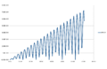
The following graph shows the total energy of the system against time at varying timestep values:

It can be seen from the graphs that for timestep = 0.001, 0.0025 and 0.0075, the energy reaches a stable equilibrium but for timestep = 0.01 and timestep = 0.015, the energy slowly decreases and rapidly increases, respectively, indicating that the results of the simulation are not very accurate for these values of timestep. Timestep = 0.015 is especially bad as it very obviously does not reach an equilibrium.

Therefore, timestep = 0.0075 would be the ideal value as it provides the highest accuracy, while running the simulation for a suitably long time to provide realistic results.

JC: Should the average total energy depend on the choice of timestep? 0.001 and 0.0025 have the same average total energy indicating that the total energy is not affected by the length of timestep for these timesteps, so 0.0025 may be a better choice.

Running Simulations Under Specific Conditions (NpT)

Temperature and Pressure Control

Pressures chosen: 2.61, 2.63

Temperatures chosen: 1.5, 1.6, 1.7, 1.8, 1.9

Timestep of 0.0025 was chosen to provide the highest accuracy possible, without shortening the simulation time too much.

In our simulation, the temperature was controlled by solving the two following equations for the instantaneous temperature $T,$ which fluctuates.

$E_K=\frac{3}{2}N{k}_{B}T$

$\frac{1}{2}\sum _i{m}_i{v}_i^2=\frac{3}{2}N{k}_{B}T(1)$

In order for $T$ to reach our target temperature $\mathfrak{𝔗},$ we introduce a constant $\gamma$ to control the velocity such that:

$\frac{1}{2}\sum _i{m}_i{\left(\gamma v_i\right)}^2=\frac{3}{2}N{k}_B\mathfrak{𝔗}(2)$

We can solve eq. $(1)$ and $(2)$ to solve for $\gamma .$

From $(2)$:

${\gamma }^2\sum _i{m}_i{v}_i^2=3N{k}_B\mathfrak{𝔗}$

Then substituting $\sum _i{m}_i{v}_i^2$ from $(1)$

${\gamma }^{2}3N{k}_{b}T=3N{k}_b\mathfrak{𝔗}$

$\gamma =\sqrt{\frac{ϵ}{T}}$

JC: Correct, but with a typo.

Examining the Input Script

To calculate the average values for our simulation, we set certain parameters for LAMMPS in the script.

fix aves all ave/time Nevery Nrepeat Nfreq

Final averages are generated on timesteps that are multiples of Nevery, for Nrepeat number of times and an average is generated every Nfreq timesteps.

In our script:

fix aves all ave/time 100 1000 100000
run 100000

The results are sampled at every 100 timesteps for 1000 times (100, 200, 300, etc.) Averages are generated every 100,000 timesteps, but our simulation runs for the same amount of time so only one average is generated from this code.

The timestep chosen for this section of the experiment was 0.0025. Therefore, the simulation was run for $100000\times 0.0025=250\text{ unit time}$

Plotting the Equations of State

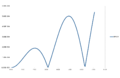
The graph above shows the density of the simulated liquid against temperature, compared with the densities derived from the ideal gas law.

It can be seen that within the ranges set for this simulation, the discrepancy between the simulated densities compared to the calculated densities are very high, to the point that the error bars for the y-axis is not even visible on the graph. Perhaps a more accurate simulation could have been run if a wider temperature and pressure ranges were selected.

With the data range being one possible source of error between the simulation and the ideal gas law prediction, another possible factor is that the parameters set for this simulation are such that the repulsive force of the Lennard-Jones interaction is more significant than the attractive force. Since the ideal gas law assumes no electronic interaction between the particles, introducing a repulsive force would result in the density of the liquid being lower than the prediction.

The most likely explanation, however, is that the ideal gas law, as its name suggests, is not very good at predicting the behavious of liquids. While both gas and liquid phases are fluids, there are major differences between them such as a much more prominent long-range order effect in liquids compared to gases.

JC: The accuracy of the simulation isn't the reason why it doesn't agree with the ideal gas law and this is not an error. An ideal gas has no interactions and particles have no volume which means that particles can be packed together to higher densities.

Calculating Heat Capacity

Graph of $C_V/V$ against Temperature

JC: What is the line that you have plotted in your graph? Have you fit it to your results?

From thermodynamics:

$C_V=\frac{\partial U}{\partial T}$

$dU=TdS-PdV$

$C_V=T\frac{\partial S}{\partial T}-P\frac{\partial V}{\partial T}$

and since $\frac{\partial S}{\partial T}\ge 0,$ heat capacity should increase with increasing temperature.

The fact that $C_V$ decreases with increasing temperature suggests that either the increase in temperature is causing the internal energy to increase at a faster rate than itself, or that there are issues with the simulation originating from possible sources such as small sampling size (number of atoms generated) or short run time.

JC: Great idea to try and explain the trend with thermodynamics. To understand this trend properly we would need to do some extra analysis looking at the density of states. What about the dependence of the heat capacity on density?

Radial Distribution Function

Looking at the graph on the right, it can be noticed that the three phases have clearly different Radial Distribution Functions (RDF) from each other. This can be attributed to the varying degrees of order each of the phases have: the atoms in the gas phase are completely free to move around, while atoms in the liquid phase have less freedom and in the solid phase, the atoms are set in a lattice, with only vibrational motion and no (or negligible) translational motion.

In order to explain the graph, let us consider the RDF to be displaying the "effective density" of atoms in an area of $\mathrm{d}\mathrm{r}$ at a distance $\mathrm{r}$ from a certain reference atom.

File:Rdf schematic.jpg

Schematic of RDF

There are three main parts to the RDF graphs: the region near the origin where the $\mathrm{R}\mathrm{D}\mathrm{F}=0$, the region after where there are big peaks and troughs, and the final region where the graphs have mostly reached equilibrium.

First of all, the region near the origin is 0 for all three phases as $\mathrm{r}$ is still within the volume (the hard sphere) of the reference atom, and hence there can be no other atoms in that radius.

The peaks in the second region indicate that there is a higher "effective density" of atoms. The explanation for this is different for the lattice structure (solid) and the fluids (liquid and gas).

For the liquid and gas phase, the peaks are due to the attractive force caused by the Lennard-Jones potential. We have calculated above (1.2 LJ Potential) that $r_{eq}=\sqrt[6]{2{\sigma }^6}.$ Setting $\sigma =1$ (as we have in our input file), we get $r_{eq}=1.122$, which is very close to where the largest peaks are for the two fluid phases.

For the solid, where all the atoms are in a lattice structure, the effects due to the Lennard-Jones interaction becomes neglibigle. Instead, there will be certain values of $\mathrm{d}\mathrm{r}$ where the effective density is higher than the overall density of the sample (the peaks), and some values of $\mathrm{d}\mathrm{r}$ where it is lower than the density of the sample (the troughs). This is arisen from the fact that as the value of $\mathrm{r}$ increases, the total volume covered by $\mathrm{d}\mathrm{r}$ also increases. But since all the atoms are set in place by the lattice, the number of atoms that $\mathrm{d}\mathrm{r}$ encompasses stays relatively constant. As a result, the peaks and the troughs tend to 1 with increasing $\mathrm{r}$.

In the case of the gas phase, the atoms are completely free to move around and the RDF graph can be entirely attributed to the effects of the L-J interaction. This justifies the lack of troughs for this phase. Furthermore, as $\mathrm{r}$ increases, the attractive part of the L-J interaction $\frac{1}{r^6}$ gets exponentially smaller and quickly becomes negligible - RDF reaches equilibrium.

Finally, the liquid phase can be considered to act as a mix between the solid phase and the gas phase: the L-J interactions are significant enough to reach equilibrium at a rate similar to the gas phase, but there exists an ordering of the atoms such that there are values of $\mathrm{r}$ where the effective density is lower than the overall density.

From the RDF of the solid phase, each of the peaks point to a certain lattice point. Simple geometrical calculations can be done to indicate that the first peak, which is the lattice point (1) closest to the reference atom (O), is at a separation of $\mathrm{r}=1.056.$ Second closest point (2) is at a distance of $\mathrm{r}=1.4938$ and the third (3) at $\mathrm{r}=1.8295.$ These points agree with the x-axis on the RDF graphs.

Face-centered cubic lattice

JC: Good explanation of the RDF and what it shows. The presence of peaks indicates ordering, so the solid has short and long range order, the liquid has only short range order and the gas is random. Did you plot the integral of the solid RDF to see how many atoms are included in the first 3 peaks?

Dynamical Properties and the Diffusion Coefficient

The Diffusion Coefficients $D$ of a simulated gas, liquid and solid were calculated using several different methods:

1) From the Mean Squared Displacement (MSD) of 8,000 simulated atoms, according to the equation $D=\frac{1}{6}\frac{\partial ⟨r^2\left(t\right)⟩}{\partial t}$

2) From the MSD of a million atoms

3) From the Velocity Autocorrelation Function (VACF), by integration.

4) From the VACF of a million atoms

The results were as follows:

Diffusion Coefficients (unit area/unit time)

Phase	From MSD	From MSD (million atoms)	From VCAF	From VCAF (million atoms)
Gas	$6.05$	$3.22$	$6.32$	$3.27$
Liquid	$0.0855$	$0.0892$	$0.0979$	$0.09$
Solid	$0.000896$	$1.5\times 10^{-5}$	$-1.66\times 10^{-5}$	$4.55\times 10^{-5}$

We can see from the table that the diffusion coefficients calculated from the same number of atoms agree very well with each other, which suggests that the results are quite precise. However, we can assume that the million atoms simulations inevitably provide more accurate data.

The results also make sense logically, where the gas have the highest diffusion coefficient (they are able to diffuse much faster) than the liquid, and the diffusion coefficient of the solid is close to 0.

Mean Squared Displacement

Graphical analysis showed that the last 1,000 timesteps are suitably linear to apply this equation, and the Diffusion Coefficients for the three different phases were found from the last 1,000 timesteps.

Velocity Autocorrelation Function

$C\left(\tau \right)=\frac{\underset{-\mathrm{\infty }}{\overset{\mathrm{\infty }}{\int }}v\left(t\right)v(t+\tau )\mathrm{d}t}{\underset{-\mathrm{\infty }}{\overset{\mathrm{\infty }}{\int }}{v}^2\left(t\right)\mathrm{d}t}$

From the 1D Harmonic Oscillator:

$x\left(t\right)=A\cos (\omega t+\varphi )$

Differentiating this gives the velocity function:

$v\left(t\right)=-A\omega \sin (\omega t+\varphi )$

Substituting this into the integrated form of the VAFC:

$C\left(\tau \right)=\frac{\underset{-\mathrm{\infty }}{\overset{\mathrm{\infty }}{\int }}A\omega \sin (\omega t+\varphi )\cdot A\omega \sin (\omega (t+\tau )+\varphi )\mathrm{d}t}{\underset{-\mathrm{\infty }}{\overset{\mathrm{\infty }}{\int }}{(A\omega \sin (\omega t+\varphi ))}^2\mathrm{d}t}$

$C\left(\tau \right)=\frac{\underset{-\mathrm{\infty }}{\overset{\mathrm{\infty }}{\int }}\sin (\omega t+\varphi )\cdot \sin (\omega (t+\tau )+\varphi )\mathrm{d}t}{\underset{-\mathrm{\infty }}{\overset{\mathrm{\infty }}{\int }}{(\sin (\omega t+\varphi ))}^2\mathrm{d}t}$

Then, from the trigonometric identity

$\sin (\alpha +\beta )=\sin \alpha \cos \beta +\sin \beta \cos \alpha ,$

$\sin (\omega t+\varphi +\omega \tau )=\sin (\omega t+\varphi )\cos \left(\omega \tau \right)+\sin \left(\omega \tau \right)\cos (\omega t+\varphi )$

$\therefore C\left(\tau \right)=\frac{\underset{-\mathrm{\infty }}{\overset{\mathrm{\infty }}{\int }}\sin (\omega t+\varphi )\cdot (\sin (\omega t+\varphi )\cos \left(\omega \tau \right)+\sin \left(\omega \tau \right)\cos (\omega t+\varphi ))\mathrm{d}t}{\underset{-\mathrm{\infty }}{\overset{\mathrm{\infty }}{\int }}{(\sin (\omega t+\varphi ))}^2\mathrm{d}t}$

$C\left(\tau \right)=\frac{\underset{-\mathrm{\infty }}{\overset{\mathrm{\infty }}{\int }}{\sin }^2(\omega t+\varphi )\cos \left(\omega \tau \right)+\underset{-\mathrm{\infty }}{\overset{\mathrm{\infty }}{\int }}\sin \left(\omega \tau \right)\cos (\omega t+\varphi )\sin (\omega t+\varphi )}{\underset{-\mathrm{\infty }}{\overset{\mathrm{\infty }}{\int }}{\sin }^2(\omega t+\varphi )}$

$\tau$ is a constant so $\cos \left(\omega \tau \right)$ and $\sin \left(\omega \tau \right)$ can be taken out of the integral.

$C\left(\tau \right)=\frac{\cos \left(\omega \tau \right)\underset{-\mathrm{\infty }}{\overset{\mathrm{\infty }}{\int }}{\sin }^{}(\omega t+\varphi )+\sin \left(\omega \tau \right)\underset{-\mathrm{\infty }}{\overset{\mathrm{\infty }}{\int }}\cos (\omega t+\varphi )\sin (\omega t+\varphi )}{\underset{-\mathrm{\infty }}{\overset{\mathrm{\infty }}{\int }}{\sin }^2(\omega t+\varphi )}$

$\underset{-\mathrm{\infty }}{\overset{\mathrm{\infty }}{\int }}{\sin }^2(\omega t+\varphi )$ can cancel out:

$C\left(\tau \right)=\cos \left(\omega \tau \right)+\frac{\sin \left(\omega \tau \right)\underset{-\mathrm{\infty }}{\overset{\mathrm{\infty }}{\int }}\cos (\omega t+\varphi )\sin (\omega t+\varphi )}{\underset{-\mathrm{\infty }}{\overset{\mathrm{\infty }}{\int }}{\sin }^2(\omega t+\varphi )}$

Since $\sin (x)$ is an odd function and $\cos (x)$ is an even function, $\sin (x)\cos (x)$ is an odd function.

$\therefore \cos (\omega t+\varphi )\sin (\omega t+\varphi )$ is an odd function (While the value of $\varphi$ can change whether or not the functions are even or odd, it shifts both functions by the same amount and the resulting $\cos (\omega t+\varphi )\sin (\omega t+\varphi )$ will still be odd)

$\therefore \underset{-\mathrm{\infty }}{\overset{\mathrm{\infty }}{\int }}\cos (\omega t+\varphi )\sin (\omega t+\varphi )=0$

$\therefore C\left(\tau \right)=\cos \left(\omega \tau \right)+\frac{\sin \left(\omega \tau \right)\underset{-\mathrm{\infty }}{\overset{\mathrm{\infty }}{\int }}\cos (\omega t+\varphi )\sin (\omega t+\varphi )}{\underset{-\mathrm{\infty }}{\overset{\mathrm{\infty }}{\int }}{\sin }^2(\omega t+\varphi )}=\cos \left(\omega \tau \right)$

$C\left(\tau \right)=\cos \left(\omega \tau \right)$

JC: Well explained derivation.

Comparison of Normalised VACF with VACF of Liquid and Solid

We can see from this graph that while the VACF of the liquid quickly decorrelates to 0, the solid still retains some minor fluctuations. This is due to the fact that the atoms in a liquid are more free to move around and collide with each other, "forgetting" what its initial velocity was from exchanging energy, whereas for atoms in the solid state, they are already in a relatively stable position (similar to $r_{eq}$ in L-J interactions) and oscillate about 0. Eventually, atoms in solids, too, will decay, but at a much slower rate than in liquids.

The VACF for the harmonic oscillator does not decay at all since the decorrelation arises from the atoms exchanging energy with their neighbours, which does not occur in harmonic oscillators.

JC: Collisions between particles cause the VACF to decorrelate, but there are no collisions in the harmonic oscillator.