Talk:Mod:PYTHONLY2412

Introduction to the Ising model

TASK1: Show that the lowest possible energy for the Ising model is $$\begin{gathered} E \\ = \\ -DNJ \end{gathered}$$, where $D$ is the number of dimensions and $N$ is the total number of spins. What is the multiplicity of this state? Calculate its entropy.

For a spin in a system of dimension $D$, there are $2D$ interactions associated with it due to its $2D$ number of neighbouring spins. To minimise the energy of these interactions, this spin and its $2D$ neighbours must have the same sign, i.e. all up or all down. Therefore the minimum energy of these interactions associated with this one spin is $$\begin{gathered} E \\ =-0.5\times 2DJ=-DJ \end{gathered}$$. If the system has total number of spins of $N$, then the overall lowest energy must be $$\begin{gathered} E \\ = \\ -DNJ \end{gathered}$$. The multiplicity of such a system should be 2 since the whole system can either have all of its spins up or down. The entropy of such a system is therefore $$\begin{gathered} S \\ = \\ {K}_b\ln 2=9.57\times 10^{-24}J{K}^{-1} \end{gathered}$$.

NJ: Very good, nice explanation.

TASK2: Imagine that the system is in the lowest energy configuration. To move to a different state, one of the spins must spontaneously change direction ("flip"). What is the change in energy if this happens ($$\begin{gathered} D=3, \\ N=1000 \end{gathered}$$)? How much entropy does the system gain by doing so?

For a system of $$\begin{gathered} D=3, \\ N=1000 \end{gathered}$$ in its lowest energy configuration, the energy of this configuration is $$\begin{gathered} E \\ =-3000J \end{gathered}$$ and the entropy of this system is $$\begin{gathered} S \\ =9.57\times 10^{-24}J{K}^{-1} \end{gathered}$$. If one of the spins change its direction, there are 6 unique interaction energies changes from -1 to +1 and the overall energy changes to $$\begin{gathered} E \\ =-2988J \end{gathered}$$. In this excited state, the entropy is $$\begin{gathered} S \\ = \\ {K}_b\ln 2000=1.05\times 10^{-22}J{K}^{-1} \end{gathered}$$ because there are 2000 ways of arranging this system. Therefore the change in energy of this process is $$\begin{gathered} \mathrm{\Delta }E \\ =12J \end{gathered}$$ and the change in entropy is $$\begin{gathered} \mathrm{\Delta }S \\ =9.54\times 10^{-23}J{K}^{-1} \end{gathered}$$.

TASK3: Calculate the magnetisation of the 1D and 2D lattices in figure 1. What magnetisation would you expect to observe for an Ising lattice with $$\begin{gathered} D=3, \\ N=1000 \end{gathered}$$ at absolute zero?

The magnetisations of the 1D and 2D lattices in figure 1 are both +1. For a Ising lattice with $$\begin{gathered} D=3, \\ N=1000 \end{gathered}$$ at absolute zero, its magnetisation can be either +1000 or -1000 because they need to be parallel to each other to minimise their energies.

NJ: all correct, very good.

Calculating the energy and magnetisation

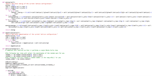
In this section, two functions from the IsingLattice.py file, energy() and magnetisation(), were completed to calculate the energy and magnetisation of any 2D Ising lattice and a screenshot of these codes is shown below in Figure 1.

Figure 1. The original code for energy() and magnetisation() functions

The validity of these two functions were checked using a given ILcheck.py file and the output is given below in Figure 2.

Figure 2. The output from the ILcheck.py file

NJ: this is all correct, but I would have liked to see some comments in the code (or in the wiki) to explain what is going on.

Introduction to Monte Carlo simulation

TASK1: How many configurations are available to a system with 100 spins? To evaluate these expressions, we have to calculate the energy and magnetisation for each of these configurations, then perform the sum. Let's be very, very, generous, and say that we can analyse $1\times 10^9$ configurations per second with our computer. How long will it take to evaluate a single value of ${⟨M⟩}_T$?

For a system of 100 spins, since each spin can be either up or down, the total number of configurations is therefore $$\begin{gathered} W \\ =2^{100}=1.27\times 10^{30} \end{gathered}$$ and it will take about $4.02\times 10^{13}$ years to calculate a single value of ${⟨M⟩}_T$.

NJ: good. Saying "about 4E13" years would have been fine too!.

TASK2: If $T<T_C$, do you expect a spontaneous magnetisation (i.e. do you expect $⟨M⟩\ne 0$)? When the state of the simulation appears to stop changing (when you have reached an equilibrium state), use the controls to export the output to PNG and attach this to your report. You should also include the output from your statistics() function.

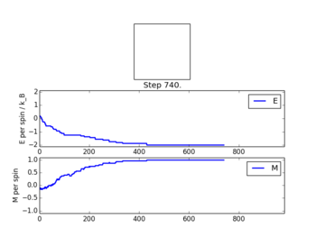
A montecarlostep(T) function and a statistics() function were written in this section to perform a single step Monte Carlo simulation and calculate average properties of the system, respectively. The output from ILanim.py file is shown below in Figure 3.

NJ: the statistics function is very good, but the montecarlostep() function is not quite right. If delta < R, you *reject* the trial move. The code you have does the opposite. The comment you have there is also not quite correct - have another read of the information about the Monte Carlo algorithm.

Figure 3. The output from ILanim.py and statistics()

NOTE: The energy in the graph above should be in the unit of J(J is the constant related to the strength of interactions between two neighboring spins), the magnetisation should be in the unit of ћ and the temperature should be in the unit of J/K_B. These units should be them same in the rest of this report unless stated otherwise.

NJ: the magnetisation is unitless — this isn't a quantum system, just a toy model. Do you expect spontaneous magnetisation below T_C?

Accelerating the code

TASK1: Use the script ILtimetrial.py to record how long your current version of IsingLattice.py takes to perform 2000 Monte Carlo steps. This will vary, depending on what else the computer happens to be doing, so perform repeats and report the error in your average!

TASK2: Use the script ILtimetrial.py to record how long your new version of IsingLattice.py takes to perform 2000 Monte Carlo steps. This will vary, depending on what else the computer happens to be doing, so perform repeats and report the error in your average!

In this section, the energy() and statistics() functions were modified using numpy.sum(), numpy.roll() and numpy.multiply() functions. After the modification, the calculation time has been shortened significantly in performing 2000 Monte Carlo steps. The comparison is shown below in Table 1.

Table 1. The effect of accelerating codes on computational time

	before acceleration	after acceleration
screen shot
average (s)	21.6	0.283
standard error (s)	0.162	0.00140

NJ: Good. Are you surprised by how big the difference is? In the magnetisation function, you don't need to do m = 0.0+np.sum(...), you can just say m = np.sum(...)

The effect of temperature

TASK1: The script ILfinalframe.py runs for a given number of cycles at a given temperature, then plots a depiction of the final lattice state as well as graphs of the energy and magnetisation as a function of cycle number. This is much quicker than animating every frame! Experiment with different temperature and lattice sizes. How many cycles are typically needed for the system to go from its random starting position to the equilibrium state? Modify your statistics() and montecarlostep() functions so that the first N cycles of the simulation are ignored when calculating the averages. You should state in your report what period you chose to ignore, and include graphs from ILfinalframe.py to illustrate your motivation in choosing this figure.

From the top picture in Figure 3, we can see that the first few hundreds step of the Monte Carlo calculation are relaxation steps. Therefore, these steps should be excluded during the calculation of average properties of the system. Some outputs from the ILfinalframe.py file for the 8x8 lattice at different temperatures are shown below in Table 2. From this table, it is clear that the first 2000 steps should be excluded and a total run-time of 50000 should be appropriate in the calculation of average proprieties of this lattice size.

Table 2. The effect of temperature on the total number of relaxation steps of the 8x8 lattice

Temperature(J/KB)	0.5	1.0
Output Screenshot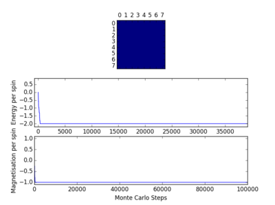
Temperature(J/KB)	1.5	2.0
Output Screenshot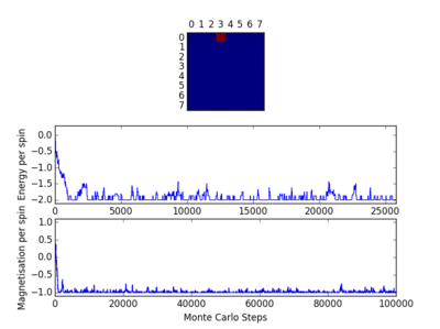

TASK: Use ILtemperaturerange.py to plot the average energy and magnetisation for each temperature, with error bars, for an $8\times 8$ lattice. Use your initution and results from the script ILfinalframe.py to estimate how many cycles each simulation should be. The temperature range 0.25 to 5.0 is sufficient. Use as many temperature points as you feel necessary to illustrate the trend, but do not use a temperature spacing larger than 0.5. T NumPy function savetxt() stores your array of output data on disk — you will need it later. Save the file as 8x8.dat so that you know which lattice size it came from.

From Table 2, it is clear that the first 2000 steps should be excluded and a total run-time of 50000 should be appropriate in the calculation of average proprieties of the 8x8 lattice. The output from the IL.temperaturerange.py file of a 8x8 lattice is shown below in Figure 4. The temperature range is from 0.2 to 5.0 and step-size is 0.1. Errors bars of average energies and magnetisations at each temperature point are shown as well. In fact these error bars are too small to be seen clearly.

Figure 4. The output from the ILtemperature.py file for 8x8 lattice

NJ: I would have liked to have seen some graphs showing how the equilibration time differs for different lattice sizes as well.

The effect of system size

TASK: Repeat the final task of the previous section for the following lattice sizes: 2x2, 4x4, 8x8, 16x16, 32x32. Make sure that you name each datafile that your produce after the corresponding lattice size! Write a Python script to make a plot showing the energy per spin versus temperature for each of your lattice sizes. Hint: the NumPy loadtxt function is the reverse of the savetxt function, and can be used to read your previously saved files into the script. Repeat this for the magnetisation. As before, use the plot controls to save your a PNG image of your plot and attach this to the report. How big a lattice do you think is big enough to capture the long range fluctuations?

The number of relaxation and equilibration steps needed to calculate reliable average properties depend strongly on the system size. Therefore, several ILfinalframe.py calculations were performed for different lattice sizes to determine the number of relaxation steps and total run-time required. The results are summarised in Table 3 below and these values are used when ILtemperaturerange.py calculations were performed for lattice sizes: 2x2, 4x4, 8x8, 16x16, 32x32.

Table 3. The relaxation and equilibration steps for different lattice sizes

lattice size	2x2	4x4	8x8	16x16	32x32
number of relaxation steps	500	1000	2000	20000	75000
total run time	20000	30000	50000	150000	300000

The ILtemperaturerange.py script was then used to calculate average energies and magnetisations of the following lattice sizes: 2x2, 4x4, 16x16, 32x32 and results are shown in Table 4.

Table 4. The output of ILtemperaturerange.py for different lattice sizes

lattice size	2x2	4x4
output
lattice size	16x16	32x32
output

Note: The temperature ranges in all the above calculations are all from 0.2 to 5.0 with the same step size 0.1.

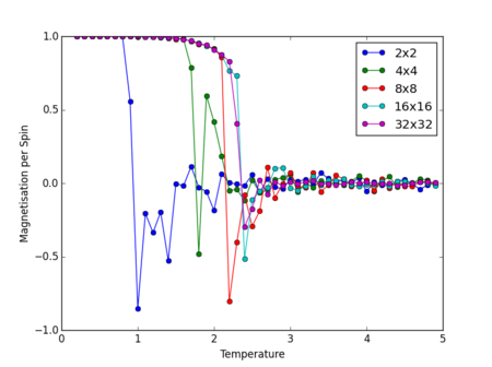
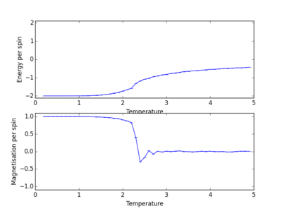
The energies and magnetisations per spin versus temperature graphs for each lattice size were then plotted together for comparisons, as shown in Figure 5.

Figure 5. The energies and magnetisations vs. temperature graphs for different lattice sizes shown in one figure

From Figure 5, it is clear to see that by increasing the lattice size from 2x2 to 4x4 and from 4x4 to 8x8, both energies and magnetisations vs. temperature curves change in shapes significantly. In other words, by increasing the lattice size from 2x2 to 8x8, the accuracy of the calculations has been greatly improved and more details of the behaviors of both energies and magnetisations vs. temperature curves have been revealed. However, by changing the lattice size from 8x8 to 16x16 and 32x32, both plots in Figure 5 do not change in general features, where as the computational time increases significantly. Therefore, the 8x8 lattice can be seen as the minimum lattice size required to capture the long range fluctuations.

NJ: Nice plots, but be careful with the wording of the explanation. The E vs T results that you get for, say, a 2x2 lattice are accurate for that lattice — it's just that a 2x2 lattice isn't a good illustration of a real ferromagnet.

Determining the heat capacity

TASK: Write a Python script to make a plot showing the heat capacity versus temperature for each of your lattice sizes from the previous section. You may need to do some research to recall the connection between the variance of a variable, $\mathrm{V}\mathrm{a}\mathrm{r}[X]$, the mean of its square $⟨X^2⟩$, and its squared mean ${⟨X⟩}^2$. You may find that the data around the peak is very noisy — this is normal, and is a result of being in the critical region. As before, use the plot controls to save your a PNG image of your plot and attach this to the report.

Since the heat capacity is defined as $C=\frac{\partial E}{\partial T}=\frac{\mathrm{V}\mathrm{a}\mathrm{r}[E]}{k_B{T}^2}$, by extracting the $⟨E^2⟩$ and $⟨E⟩$ data from the .dat files generated previously, heat capacity versus temperature curves for each lattice size were computed and plotted in Figure 6.

Figure 6. Heat capacity versus temperature curves for all the lattice sizes

NOTE: The heat capacity in the graph above has the unit of K_B and it has the same unit in the rest of this report.

In Figure 6, as lattice size increases, the temperature as which maximum heat capacity occurs shifts to the left gradually. This is expected due to the finite size effect, which is very common in the simulations of systems bearing long ranged interactions. The trend in Figure 6 is actually in good agreement with the relationship $T_{C,L}=\frac{A}{L}+T_{C,\mathrm{\infty }}$, where $T_{C,L}$ is the Curie temperature of an $L\times L$lattice, $T_{C,\mathrm{\infty }}$ is the Curie temperature of an infinite lattice, and $A$ is a constant.

NJ: There aren't any long range interaction in this system. Each spin interacts only with its four nearest neighbours. There are long range correlations when you get close to the critical point. NJ: It would be good to explicitly point out that you've calculated the heat capacity per spin

Locating the Curie temperature

TASK1: A C++ program has been used to run some much longer simulations than would be possible on the college computers in Python. You can view its source code here if you are interested. Each file contains six columns: $T,E,E^2,M,M^2,C$ (the final five quantities are per spin), and you can read them with the NumPy loadtxt function as before. For each lattice size, plot the C++ data against your data. For one lattice size, save a PNG of this comparison and add it to your report — add a legend to the graph to label which is which. To do this, you will need to pass the label="..." keyword to the plot function, then call the legend() function of the axis object (documentation here).

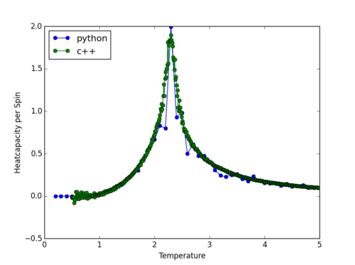
The heat capacity versus temperature curves calculated using data generated by Phthon and C++ for the 32x32 lattice is plotted in Figure 7. The two curves coincide with each other in both the low and high temperature regions. However, in the central peak region, the C++ curve is more continuous as it contains more points. i.e. The C++ curve has a better resolution in the peak region.

NJ: The C++ code has better resolution everywhere, because the temperature spacing used was much smaller.

Figure 7. Comparisons between heat capacity calculated from C++ and Python data for the lattice size of 32x32

TASK2: write a script to read the data from a particular file, and plot C vs T, as well as a fitted polynomial. Try changing the degree of the polynomial to improve the fit — in general, it might be difficult to get a good fit! Attach a PNG of an example fit to your report.

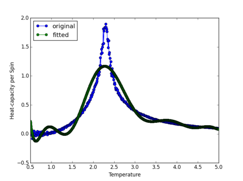
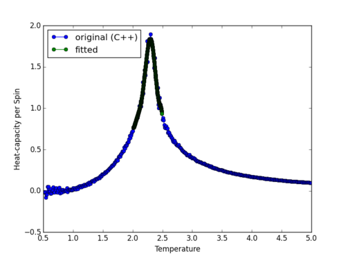
A 10th order polynomial was fitted to the C++ heat capacity curve for the 32x32 lattice, shown in Figure 8. However, this is still not a good fit, as it cannot capture the peak region accurately.

Figure 8. Fitting 10th order polynomial to the heat capacity curve obtained from C++ data with lattice size of 32x32

TASK3: Modify your script from the previous section. You should still plot the whole temperature range, but fit the polynomial only to the peak of the heat capacity! You should find it easier to get a good fit when restricted to this region.

An 8th order polynomial was then fitted to the peak region of the C++ curve for the 32x32 lattice(between 2.0 and 2.5 K), as shown in Figure 9. The area around the Curie temperature is successfully mimicked in Figure 9 and from this graph, $T_{C,32}$ can be extracted successfully. If the order of the polynomial was increased even higher, an error message would pop up to alert about the possible poor quality of the polynomial fitting.

NJ: Nice fits. If a fitting program warns you about poor fitting, it's usually only guidance. Use your best judgment!

Figure 9. Fitting 8th order polynomial to the peak region of the heat capacity curve obtained from C++ data with lattice size of 32x32

TASK4: find the temperature at which the maximum in C occurs for each datafile that you were given. Make a text file containing two colums: the lattice side length (2,4,8, etc.), and the temperature at which C is a maximum. This is your estimate of $T_C$ for that side length. Make a plot that uses the scaling relation given above to determine $T_{C,\mathrm{\infty }}$. By doing a little research online, you should be able to find the theoretical exact Curie temperature for the infinite 2D Ising lattice. How does your value compare to this? Are you surprised by how good/bad the agreement is? Attach a PNG of this final graph to your report, and discuss briefly what you think the major sources of error are in your estimate.

By doing the polynomial fitting described earlier to all the lattice sizes, $T_{C,L}$ for all the lattice sizes were obtained and summarised in Table 5 below. $T_{C,L}$ was then plotted against $1/L$ to find $T_{C,\mathrm{\infty }}$, as shown in Figure 10.

Table 5. $T_{C,L}$ for all the lattice sizes

lattice size	2x2	4x4	8x8	16x16	32x32	64x64
$T_C$(J/KB)	2.52830831	2.45439439	2.34848849	2.30837838	2.29540541	2.27378378

Figure 10. $T_C$ against $1/L$ curve

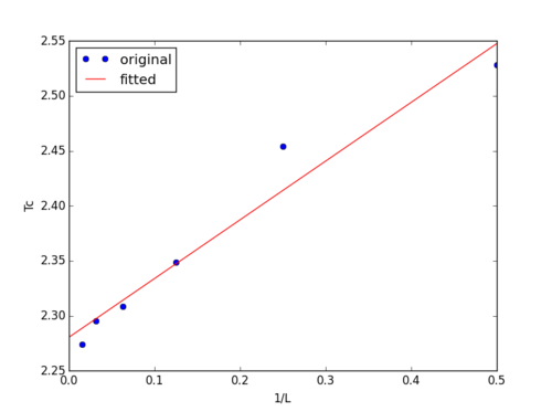
The straight line in Figure 10 was obtained by fitting a first order polynomial to the $T_C$ vs. $1/L$ data. The y-intercept of this line is 2.281 J/K_B, which is slightly higher than the theoretical Curie Temperature for the infinite 2D Ising lattice, 2.269 J/K_B.

The reasons behind the difference between the value obtained via this computational exercise and the theoretical value may be threefold.

1. The lack of data points on the right hand side of the graph due to the nature of the x-axis which is 1/L and L must be integers. Therefore, only three points are possible to be located on the right half of the graph with x coordinates, 0.25, 0.33 and 0.5.

2. The qualities of the $T_C$ values for small lattices such as 2X2 and 4x4 are poor. There are only 4 spins in the 2x2 lattice, which means the possible values of the energy and the magnetisation of the system are very limited. Therefore the variance of the energy of this system can very significantly from one simulation to another, especially in the region near the Curie temperature, which means $T_C$ can vary from one simulation to another.

3. The order of the polynomial and the exact peak region that we chose to fit the polynomial onto can greatly influence the $T_C$ values obtained.

One way of improving the accuracy of the Curie temperature found using this method may be neglecting the data for 2x2 and 4x4 lattices, and including more larger lattices such as 128x128 and 256x256. The drawback of simulating a even larger Ising lattice is obvious as it is very computationally demanding.In fact, the $T_C$ found using the 64x64 lattice is closer to the theoretical value than the one obtained from linear fit. Therefore, the $T_C$ found using a 256x256 lattice could probably be approximated as $T_{C,\mathrm{\infty }}$ already, because the constant A would have been scaled down by 256 times and thus cause very little influence to the $T_{C,\mathrm{\infty }}$.

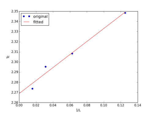
Actually, just by ignoring the data from 2x2 and 4x4 lattices, and fitting a straight line to the rest of the points, a much better result is obtained, as shown in Figure 11. In Figure 11, the y-intercept is exactly 2.269 J/K_B. However, the quality of this analysis is highly questionable due to the fact that only 4 points are used.

NJ: Very good - well done for spotting that you can ignore the 2x2 and 4x4 points.

Figure 11. $T_C$ against $1/L$ curve

References

- ↑ H.A. Kramers and G.H. Wannier, Phys. Rev. 60, 252 (1941).