Talk:Mod:MLLS17

JC: General comments: Most tasks answered well, make sure your plots are clear and use multiple plots if it is clearer. Make sure you understand the background theory behind each task and can use that to explain your results.

Molecular dynamics simulations of simple liquids

Many chemical phenomena are studies using computer simulations. Molecular dynamic simulations is a method for studying the physical movements of atoms and molecules. The atoms and molecules are left to interact in given conditions for a set period of time and the dynamic evolution of the system is studied. Practically this can be used to monitor the behavior of protein folding and properties of biological systems such as lipid membranes.

Introduction to molecular dynamic simulations

The Velocity-Verlet Algorithm

In the classical particle approximation the Schrodinger equation is used to describe the behavior of any particular chemical system. The limitation to this method is that for anything more complicated than a hydrogen atom, the behavior of the system cannot be solved exactly. Even approximated solutions can be computationally demanding.

In the velocity-verlet Algorithm rather than treating the atomic positions, velocities and forces as continuous functions of time, we break our simulation up into a sequence of timesteps, each of length $\delta t$.

In this exercise the equation of the position of the classical harmonic oscillator $x\left(t\right)=A\cos (\omega t+\varphi )$ was calculated as the 'analytical' values. These values were then compared to the values calculated using the velocity-verlet algorithm.

	molecule1
Figure 1: Classical solution for the position (analytical values) against time	Figure 2: Total energy of the velocity-verlet solution against time
molecule1
Figure 3: Absolute difference between analytical values and velocity-verlet solution against time

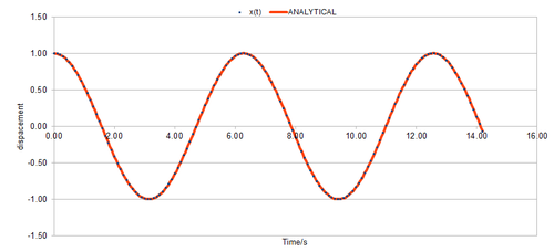
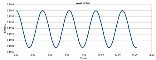
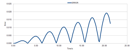
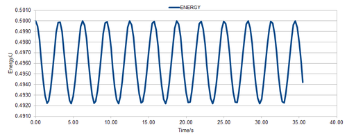
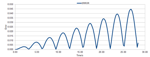
Figure 1 shows the classical harmonic oscillator solution of the position ("ANALYTICAL") against the time using $A=\omega =1$ and $\varphi =0$. Figure 2 shows the energy against time in which the energy was calculated using the equation $$\begin{gathered} E=\frac{1}{2} \\ m \\ {v}^2+\frac{1}{2} \\ k \\ {x}^2 \end{gathered}$$ which is the kinetic and potential energy of the system respectively. The $v$ and $x$ values were calculated using the velocity-Verlet algorithm. Figure 3 shows the error against time where the error is the absolute difference between the "ANALYTICAL" and the velocity-Verlet solution. The position of the classical harmonic oscillator is given by $x\left(t\right)=A\cos (\omega t+\varphi )$.

For the default timestep value, 0.1, estimate the positions of the maxima in the ERROR column as a function of time. Make a plot showing these values as a function of time, and fit an appropriate function to the data.

The error of the values between the velocity-Verlet and classical oscillator approximated values of the position of particles increased along with the time steps. This can be seen on figure 3 where the plot of the positions of maximum error has been plotted against time.

JC: Why does the error oscillate?

What sort of a timestep do you need to use to ensure that the total energy does not change by more than 1% over the course of your "simulation"? Why do you think it is important to monitor the total energy of a physical system when modelling its behaviour numerically?

molecule1	molecule1
Figure 4: Total energy of the velocity-verlet solution against time with timestep = 0.15	Figure 7: The error sgainst time with timesteps = 0.15
molecule1	molecule1
Figure 5: Total energy of the velocity-verlet solution against time with timestep = 0.25	Figure 8: The error sgainst time with timesteps = 0.25
molecule1	molecule1
Figure 6: Total energy of the velocity-verlet solution against time with timestep = 0.20	Figure 9: The error sgainst time with timesteps = 0.20

Figures 4, 5 and 6 shows the energy calculated using the velocity-Verlet solution against time for timesteps 0.15, 0.25 and 0.20 respectively. It showed that as the timestep increased the difference in energy between the maxima and the minima of energy increased and hence the percentage error of the energy also increased. This face is reiterated in figures 7,8 and 9 where it can be seen that the maximum error values become more frequent and greater as the timestep increases.

An estimation of the percentage error of the energy over the time of the simulation is shown on the table figure 10.

molecule1
Figure 10

Figure 10 shows a few of the percentage errors that were calculated. It can be seen that a timestep of 0.002 is needed for the total energy to not change over 1%.

It is important to monitor the total energy of a physical system when modelling its behaviour numerically because it can be indicative of whether the law of conservation energy is in action and also that the system is in thermal equilibrium. Both these must be met so that the behavior of the system can be calculated and compared to other systems numerically. The numerical thermodynamic properties derived from these values will be different if the law of conservation energy and thermal equilibrium are not met.

JC: Good choice of timestep and explanation - assuming you mean 0.2?

Atomic force and the Lennard Jones Potential

The forces acting on a given configuration fo atoms cannot be reasonably solved using quantum physics equations. Therefore approximations must be made. In classical physics the force acting on an object is determined by the potential that it experiences.

${\mathbf{F}}_i=-\frac{\mathrm{d}U\left({\mathbf{r}}^N\right)}{\mathrm{d}{\mathbf{r}}_i}$

The function U defines all the key physics of interatomic interactions in a system. The Lennard Jones potential can be used to model the interactions between each pair of atoms. Overall U is given by the equation;

$U\left({\mathbf{r}}^N\right)=\sum _i^N\sum _{i\ne j}^N\left\{4ϵ(\frac{{\sigma }^{12}}{r_{ij}^{12}}-\frac{{\sigma }^6}{r_{ij}^6})\right\}$

1. For a single Lennard-Jones interaction, $\varphi \left(r\right)=4ϵ(\frac{{\sigma }^{12}}{r^{12}}-\frac{{\sigma }^6}{r^6})$, find the separation, $r_0$, at which the potential energy is zero

$\varphi \left(r\right)=4ϵ(\frac{{\sigma }^{12}}{r^{12}}-\frac{{\sigma }^6}{r^6})=0$ $\frac{{\sigma }^{12}}{r^{12}}-\frac{{\sigma }^6}{r^6}=0$ $\frac{{\sigma }^{12}}{r^{12}}=\frac{{\sigma }^6}{r^6}$ ${\sigma }^6=r^6$ $\sigma =r_0$

Therefore the phase separation $r_0$ is $\sigma$ when the potential energy is zero.

2. What is the force at this separation?

${\mathbf{F}}_i=-\frac{\mathrm{d}U\left({\mathbf{r}}^N\right)}{\mathrm{d}{\mathbf{r}}_i}$ $U\left({\mathbf{r}}^N\right)=\sum _i^N\sum _{i\ne j}^N\left\{4ϵ(\frac{{\sigma }^{12}}{r_{ij}^{12}}-\frac{{\sigma }^6}{r_{ij}^6})\right\}$

Therefore

${\mathbf{F}}_i=-\frac{\mathrm{d}}{dr}\sum _i^N\sum _{i\ne j}^N\left\{4ϵ(\frac{{\sigma }^{12}}{r_{ij}^{12}}-\frac{{\sigma }^6}{r_{ij}^6})\right\}$ ${\mathbf{F}}_i=-\sum _i^N\sum _{i\ne j}^N\left\{4ϵ(\frac{-12{\sigma }^{12}}{r_{ij}^{13}}+\frac{6{\sigma }^6}{r_{ij}^7})\right\}$

$\sigma =r_0$ as $U\left({\mathbf{r}}^N\right)=0$

${\mathbf{F}}_i=\{-4ϵ(\frac{-12}{\sigma }+\frac{6}{\sigma })\}$ ${\mathbf{F}}_i=\frac{24ϵ}{\sigma }$

The force at the separation where the potential energy is zero is therefore $\frac{24ϵ}{\sigma }$.

3. Find the equilibrium separation, $r_{eq}$, and work out the well depth ($\varphi \left(r_{eq}\right)$) $\frac{\mathrm{d}U\left({\mathbf{r}}^N\right)}{\mathrm{d}{\mathbf{r}}_i}=0$

This is a stationary point in the Lennard Jones potential.

$-4ϵ(\frac{-12{\sigma }^{12}}{r^{13}}-\frac{6{\sigma }^6}{r^7})=0$ $\frac{12{\sigma }^{12}}{r^{13}}=\frac{6{\sigma }^6}{r^7}$ $2{\sigma }^6=r^6$ $r_{(}eq)=2^{\frac{1}{6}}\sigma$

Then for the well depth

$U\left({{\mathbf{r}}_{\mathbf{(}}\mathbf{e}\mathbf{q}\mathbf{)}}^N\right)=\sum _i^N\sum _{i\ne j}^N\left\{4ϵ(\frac{{\sigma }^{12}}{4{\sigma }^{12}}-\frac{{\sigma }^6}{2{\sigma }^6})\right\}$ $U\left({{\mathbf{r}}_{\mathbf{(}}\mathbf{e}\mathbf{q}\mathbf{)}}^N\right)=\sum _i^N\sum _{i\ne j}^N\left\{4ϵ(\frac{1}{4}-\frac{1}{2})\right\}$ $U\left({{\mathbf{r}}_{\mathbf{(}}\mathbf{e}\mathbf{q}\mathbf{)}}^N\right)=-ϵ$

Therefore at equilibrium distance the well depth is equal to $-ϵ$.

4. Evaluate the integrals $\underset{2\sigma }{\overset{\mathrm{\infty }}{\int }}\varphi \left(r\right)\mathrm{d}r$, $\underset{2.5\sigma }{\overset{\mathrm{\infty }}{\int }}\varphi \left(r\right)\mathrm{d}r$, and $\underset{3\sigma }{\overset{\mathrm{\infty }}{\int }}\varphi \left(r\right)\mathrm{d}r$ when $\sigma =ϵ=1.0$.

$\int \varphi \left(r\right)\mathrm{d}r=\int 4ϵ(\frac{{\sigma }^{12}}{r^{12}}-\frac{{\sigma }^6}{r^6})\mathrm{d}r=4ϵ(\frac{{\sigma }^{12}}{-11r^{11}}-\frac{{\sigma }^6}{-5r^5})$

4.1 $\underset{2\sigma }{\overset{\mathrm{\infty }}{\int }}\varphi \left(r\right)\mathrm{d}r=4ϵ(\frac{{\sigma }^{12}}{-11r^{11}}-\frac{{\sigma }^6}{-5r^5}){|}_{2\sigma }^{\mathrm{\infty }}==0-4ϵ(\frac{{\sigma }^{12}}{-11{\left(2\sigma \right)}^{11}}-\frac{{\sigma }^6}{-5{\left(2\sigma \right)}^5})=-0.0248(3.s.f)$

4.2 $\underset{2.5\sigma }{\overset{\mathrm{\infty }}{\int }}\varphi \left(r\right)\mathrm{d}r=4ϵ(\frac{{\sigma }^{12}}{-11r^{11}}-\frac{{\sigma }^6}{-5r^5}){|}_{2.5\sigma }^{\mathrm{\infty }}=0-4ϵ(\frac{{\sigma }^{12}}{-11{\left(2.5\sigma \right)}^{11}}-\frac{{\sigma }^6}{-5{\left(2.5\sigma \right)}^5})=-0.00818(3.s.f)$

4.3 $\underset{3\sigma }{\overset{\mathrm{\infty }}{\int }}\varphi \left(r\right)\mathrm{d}r=4ϵ(\frac{{\sigma }^{12}}{-11r^{11}}-\frac{{\sigma }^6}{-5r^5}){|}_{3\sigma }^{\mathrm{\infty }}=0-4ϵ(\frac{{\sigma }^{12}}{-11{\left(3\sigma \right)}^{11}}-\frac{{\sigma }^6}{-5{\left(3\sigma \right)}^5})=-0.00329(3.s.f)$

when $\sigma =ϵ=1.0$

JC: All maths correct and clearly laid out.

The integral of the Lennard Jones potential corresponds to the force interaction between two atoms. The different integral boundary conditions shows that as the difference between the upper an lower boundary condition increases the force interaction between the two atoms tends to zero. This illustrates how as the distance between two atoms increases the interaction decreases.

JC: The force is the derivative of the potential, not the intergal.

Periodic boundary conditions

The tasks will illustrate why it is not possible to simulate realistic volumes of liquid, with the number of atom,$N$ between $1000$ and $10000$.

1. Estimate the number of water molecules in 1 ml of water under standard conditions.

Density of water = $1\frac{g}{c{m}^3}$ Molar mass of water = $18\frac{g}{mo{l}^{-1}}$

Mass of water in 1 mL = $1\frac{g}{c{m}^3}\times 1mL=1g$ Therefore the number of moles in 1 mL = $\frac{1}{18}mol$

Number of water molecules in 1 mL = $6.023\times 10^{23}\times \frac{1}{18}mol=3.35\times 10^{22}(3.s.f)$

2. Estimate the volume of $10000$ water molecules under standard conditions.

Using the previous task if there are $3.35\times 10^{22}$ water molecule in 1 mL, 10000 water molecules occupy a volume of $1mL\times \frac{10000}{3.35\times 10^{22}}=2.99\times 10^{-19}mL(3.s.f)$

In 1mL of water which is a volume that an be used in labs and hence is considered realistic. However as calculated there are far too many water molecules to simulate all of them. Even when simulating 10,000 water molecules this only represents $2.99\times 10^{-19}mL$ which is not a realistic volume.

3. Consider an atom at position $(0.5,0.5,0.5)$ in a cubic simulation box which runs from $(0,0,0)$ to $(1,1,1)$. In a single timestep, it moves along the vector $(0.7,0.6,0.2)$. At what point does it end up, after the periodic boundary conditions have been applied?.

Position before periodic boundary conditions applied = $(0.5,0.5,0.5)+(0.7,0.6,0.2)=(1.2,1.1,0.7)$

Position after periodic boundary conditions applied = $(0.2,0.1,0.7)$

The atoms are enclosed in a box of fixed dimensions. The periodic boundary condition is applied to ensure that when an atom passes out the boundary another atom passes through into the boundary so that the number of atoms in the box stays constant.

Reduced units

When using the Lennard Jones potential reduced units are used in order to make the values more manageable.

The Lennard-Jones parameters for argon are $$\begin{gathered} \sigma =0.34\mathrm{n}\mathrm{m},ϵ \\ / \\ {k}_B=120\mathrm{K} \end{gathered}$$. 1. If the LJ cutoff is $r^{*}=3.2$, what is it in real units?

distance $r^{*}=\frac{r}{\sigma }$

$r=3.2\times 0.34\times 10^{-9}=1.09\times 10^{-9}m=1.09nm$

2. What is the well depth in $$\begin{gathered} {\mathrm{k}\mathrm{J} \\ \mathrm{m}\mathrm{o}\mathrm{l}}^{-1} \end{gathered}$$?

energy $E^{*}=\frac{E}{ϵ}$

$U\left({{\mathbf{r}}_{\mathbf{(}}\mathbf{e}\mathbf{q}\mathbf{)}}^N\right)=-ϵ$

Therefore

$ϵ=-120K\times 1.38\times 10^{-23}=1.66\times 10^{-21}J(3.s.f)=0.997KJ/mol$

3. What is the reduced temperature $T^{*}=1.5$ in real units?

temperature $T^{*}=\frac{k_{B}T}{ϵ}$

$T=\frac{1.5\times 1.66\times 10^{-21}}{1.38\times 10^{-23}}=180K$

JC: All calculations correct and working clearly shown.

Equilibration

Creating the simulation box

In order to start a simulation the initial states of all the atoms in the system must be known. For a crystal this would be straight forward however generating coordinates for a liquid is more difficult. There is no long range order therefore there cannot be a reference point in order to work out the points of all the other atoms. We could create random positions for each atom however this may cause problems.

1. Why do you think giving atoms random starting coordinates causes problems in simulations? Hint: what happens if two atoms happen to be generated close together? This may cause problems because if two atoms happen to be generated close together the coordinates could overlap. This will cause problems with defining some properties of the atoms.

JC: Be more specific. Overlapping atoms will cause high repulsive forces which make the simulation unstable and can cause it to crash.

2. Satisfy yourself that this lattice spacing corresponds to a number density of lattice points of $0.8$.

$\text{Volume}=1.07722^3=1.25uni{t}^3$

$\text{Number density}=\frac{\text{Number of lattice points per unit cell}}{\text{Unit volume}}=\frac{1}{1.25}=0.8(1.d.p)$

3. Consider instead a face-centred cubic lattice with a lattice point number density of 1.2. What is the side length of the cubic unit cell?

$1.2=\frac{\text{Number of lattice points per unit cell}}{\text{Unit volume}}=\frac{4}{V}$

$\text{Volume of cubic unit cell}=\frac{4}{1.2}$

$\text{Side Length of the cubic unit cell}=\sqrt[3]{\frac{4}{1.2}}=1.49(3.s.f)$

4. Consider again the face-centred cubic lattice from the previous task. How many atoms would be created by the create_atoms command if you had defined that lattice instead?

A simple cubic lattice has one lattice point per unit cell whereas a face-centred cubic lattice has 4 lattice points per unit cell. Therefore if in the simple cubic lattice 1 box creates 1000 atoms in a face-centered lattice 1 box will create 4000 atoms.

JC: Correct.

Setting the properties of the atom

The physical properties of the atoms must also be known as well as their positions in order to perform the simulations. For the simulations all the atoms are set with the same mass and same.

1. Find the purpose of the following commands in the input script:

mass 1 1.0
pair_style lj/cut 3.0
pair_coeff * * 1.0 1.0

mass 1 1.0: This line is defining an atom of type 1 with a mass 1.0.

pair_style lj/cut 3.0: This is a set of formula(s) used to compute pairwise interactions. In LAMMPS, the pair potential is defined within a cutoff distance and the set of active interactions change over time. Therefore this code defines the cutoff as a distance of 3.0.

pair_coeff * * 1.0 1.0: Specifies the pair wise force field interaction for one or more atom types. The two asterisks correspond to two atoms of any type in the system. The two numbers at the end correspond to two coefficients in this case $\sigma =ϵ=1.0$.

JC: Why do we use a cutoff for the potential?

So far we have said that there are 1000 atoms in the box and the starting position for all the atoms are defined. We have also set all their masses and calculated the interaction between pairs of atoms. We have to finally specify the velocity of each atom.

At equilibrium the velocities of the atoms are distributed by the Maxwell-Boltzmann distribution. The velocity can be found if the masses and and temperature of simulation is known.

Running the simulation

1. Given that we are specifying ${\mathbf{x}}_i\left(0\right)$ and ${\mathbf{v}}_i\left(0\right)$, which integration algorithm are we going to use?

### SPECIFY TIMESTEP ###
variable timestep equal 0.001
variable n_steps equal floor(100/${timestep})
timestep ${timestep}

### RUN SIMULATION ###
run ${n_steps}
run 100000

With a timestep of 0.001, run ${n_steps} is used to calculate how many runs to carry out. It is more efficient to set the number of runs to 100000, especially when running simulations at several different timesteps.

JC: Why is it better to use variables to define the values of simulation parameters? In this case what happens if we want to change the timestep?

Checking equilibration

1. Make plots of the energy, temperature, and pressure, against time for the 0.001 timestep experiment.

molecule1	molecule1
Figure 11: A plot of total energy against time for a 0.001 timestep experiment	Figure 12: A plot of temperature against time for a 0.001 timestep experiment
molecule1
Figure 13: A plot of the pressure against time for a 0.001 timestep experiment

2. Does the simulation reach equilibrium? How long does this take?

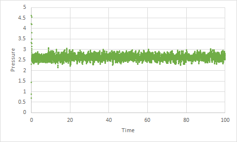
Figure 11, 12 and 13 show that the simulations for Total energy, temperature and time all reach equilibrium rapidly. The total energy reaches equilibrium at approximately -3.184 at time 0.38. The temperature reaches equilibrium at approximately 1.24 at time 0.27. The pressure reaches equilibrium at approximately 2.6 at time 0.17.

3. When you have done this, make a single plot which shows the energy versus time for all of the timesteps (again, attach a picture to your report).

molecule1
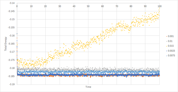
Figure 14: Total energy against time for varying timesteps

4. Choosing a timestep is a balancing act: the shorter the timestep, the more accurately the results of your simulation will reflect the physical reality; short timesteps, however, mean that the same number of simulation steps cover a shorter amount of actual time, and this is very unhelpful if the process you want to study requires observation over a long time. Of the five timesteps that you used, which is the largest to give acceptable results? Which one of the five is a particularly bad choice? Why?

It can be seen on figure 14 for timesteps 0.015, 0.01 and 0.0075 the thermal equilibrium is not reached within the timescale. For timestep 0.015 there is a constant increase therefore is a particularly bad choice. For timestep 0.01 an 0.0075 there is a constant decrease therefore is not an acceptable timestep to use. For timesteps 0.001 and 0.0025, the equilibrium is reached within the timescale of the simulation. Out of these 0.001 will give more accurate results for the simulation. On the other hand the timestep 0.0025 will be useful for observing the system for a larger period of time.

JC: The energy for 0.01 and 0.0075 looks roughly constant, but these timesteps are not suitable because the average energy should not depend on the choice of timestep. 0.0025 and 0.001 give the same average energy, so choose 0.0025 so that the simulation can cover more time.

Running simulations under specific conditions

Ensembles are used in statistical thermodynamics to describe different sorts of experimental conditions. A chemists we often use the isobaric-isothermal ensemble. In this section we are going to run simulations under the NpT conditions and sketch an equation of state for our model fluid at atmospheric pressure.

Thermostats and Barostats

We need to choose $\gamma$ so that the temperature is correct $T=\mathfrak{𝔗}$ if we multiply every velocity $\gamma$.

The equipartition theorem in statistical thermodynamics states that on average, every degree of freedom in a system at equilibrium will have $\frac{1}{2}{k}_{B}T$ of energy. In the system if there are $N$ atoms, each with 3 degrees of freedom therefore we can write two equations:

$E_K=\frac{3}{2}N{k}_{B}T$

$\frac{1}{2}\sum _i{m}_i{v}_i^2=\frac{3}{2}N{k}_{B}T$

Solve these to determine $\gamma$.

$\frac{1}{2}\sum _i{m}_i(v_i\gamma {)}^2=\frac{3}{2}N{k}_B\mathfrak{𝔗}$

This equation shows the modified velocity to give the desired energy from the target temperature.

${\gamma }^2\frac{1}{2}\sum _i{m}_i(v_i{)}^2=\frac{3}{2}N{k}_B\mathfrak{𝔗}$

${\gamma }^2\frac{3}{2}N{k}_{B}T=\frac{3}{2}N{k}_B\mathfrak{𝔗}$

Therefore

$\gamma =\pm \sqrt{\frac{\mathfrak{𝔗}}{T}}$

$\gamma$ changes varies depending on whether the kinetic energy of the system is too high or low. If the kinetic energy and temperature is higher than the target energy and temperature $\gamma$ must be lowered and vice versa.

JC: Correct. Take the positive root since gamma should only scale the magnitude of the velocities, not reverse them.

Examining the Input Script

1. What is the importance of the three numbers 100 1000 100000. How often will values of the temperature, etc., be sampled for the average? How many measurements contribute to the average?

fix aves all ave/time 100 1000 100000 v_dens v_temp v_press v_dens2 v_temp2 v_press2

The three numbers 100, 1000 and 100000 represent Nevery, Nrepeat and Nfreq respectively. It defines the timesteps of the input values that will be used for the average.

Nevery: The spacing between the timestep values that will be used in the average.

Nrepeat: How many input values will be chosen to calculate the average.

Nfreq: The calculation of averages every Nfreq timestep.

The temperature for the average will be sampled every 100000 timestep with a 100 timestep interval. 1000 measurements contribute to the average.

2. Looking to the following line, how much time will you simulate?

$\text{Total time}=100000\times 0.0025=250\text{time units}$

Plotting the equations of state

1. Choose 5 temperatures (above the critical temperature $T^{*}=1.5$), and two pressures.

$T^{*}=1.5,1.6,1.7,1.8,1.9$

$P=2.6,2.7$

A timestep of 0.0025 was chosen on the basis of the results from the previous seciton.

molecule1	molecule1
Figure 11: Density against reduced temperature with standard error error bars	Figure 12: Density against temperature comparative to the ideal gas derived values

The plot shows that as the temperature increase the density decreases which is due to the expansion of the material. As the systems is heated the particles will gain kinetic energy which will cause more frequent collisions with the wall. Despite the more frequent collisions the pressure stays constant. This shows that the surface area of the walls has increased hence the volume increased and density decreased.

By combining the simulation results and the theoretical values derived from the ideal gas equation it can be seen that the simulated density is much lower. This is because the ideal gas theory assumes that there are no interactions between the particles. With this assumption the particles are able to be much closer together in the system hence would have much higher densities. Although there are attractive and repulsive interactions within a non-ideal system the repulsive forces have a greater contribution than the attractive forces therefore overall the repulsive forces will cause the system to be less dense than the ideal gas system. The ideal gas theory only works in low-density and hence low pressure systems where the interaction between the particles are minimal. Therefore as the pressure increases and the system becomes denser the discrepancy between the ideal gas derived values and the simulations would increase.

JC: Good explanation, the discrepancy with results also gets smaller as temperature increases. Why have you fitted a straight line to the ideal gas results? The ideal gas equation shows that density is proportional to 1/T.

Calculating heat capacities using statistical physics

Heat capacity calculations

1. Run simulations at ten phase points. In this section, we will be in density-temperature $({\rho }^{*},T^{*})$ phase space, rather than pressure-temperature phase space. The two densities required at $0.2$ and $0.8$, and the temperature range is $2.0,2.2,2.4,2.6,2.8$.

Densities: 0.2, 0.8

Temperatures: 2.0, 2.2, 2.4, 2.6, 2.8

2. Plot $C_V/V$ as a function of temperature, where $V$ is the volume of the simulation cell, for both of your densities. Is the trend the one you would expect?

molecule1
Figure 13: $C_V/V$ as a function of temperature of two densities

Figure 13 shows how the Heat Capacity/Volume of simulating cell varies with temperature for densities 0.2 and 0.8. For both densities the Heat Capacity/Volume decreases as the temperature increases.

The equation of the heat capacity of an ideal gas is derived from statistical thermodynamics as:

$C_{\text{V}}={\left(\frac{\partial U}{\partial T}\right)}_{\text{V}}=\frac{3}{2}nR$

$PV=nRT$

$\frac{PV}{T}=nR$

$C_{\text{V}}=\frac{3}{2}\frac{PV}{T}$

$\frac{C_{\text{V}}}{V}=\frac{3}{2}\frac{P}{T}$

The Pressure is constant therefore in theory $\frac{C_{\text{V}}}{V}$ and Temperature is inversely proportional which is was is observed.

JC: What function have you used to fit the heat capacity data? Can you explain why the heat capacity is higher at higher density?

3. Attach an example of one of your input scripts to your report.

### DEFINE DENSITY ###
variable density equal 0.2


### DEFINE SIMULATION BOX GEOMETRY ###
lattice sc ${density}
region box block 0 15 0 15 0 15
create_box 1 box
create_atoms 1 box

### DEFINE PHYSICAL PROPERTIES OF ATOMS ###
mass 1 1.0
pair_style lj/cut/opt 3.0
pair_coeff 1 1 1.0 1.0
neighbor 2.0 bin

### SPECIFY THE REQUIRED THERMODYNAMIC STATE ###
variable T equal 2.0 
variable timestep equal 0.0025 

### ASSIGN ATOMIC VELOCITIES ###
velocity all create ${T} 12345 dist gaussian rot yes mom yes

### SPECIFY ENSEMBLE ###
timestep ${timestep}
fix nve all nve 

### THERMODYNAMIC OUTPUT CONTROL ###
thermo_style custom time etotal temp press
thermo 10

### RECORD TRAJECTORY ###
dump traj all custom 1000 output-1 id x y z

### SPECIFY TIMESTEP ###

### RUN SIMULATION TO MELT CRYSTAL ###
run 10000
unfix nve
reset_timestep 0

### BRING SYSTEM TO REQUIRED STATE ###
variable tdamp equal ${timestep}*100
fix nvt all nvt temp ${T} ${T} ${tdamp} 
run 10000
unfix nvt
fix nve all nve 
reset_timestep 0

### MEASURE SYSTEM STATE ###
thermo_style custom step etotal temp atoms vol
variable eng equal etotal
variable eng2 equal etotal*etotal
variable temp equal temp
variable temp2 equal temp*temp
variable n equal atoms
variable n2 equal atoms*atoms
variable vol equal vol
fix aves all ave/time 100 1000 100000 v_eng v_eng2 v_temp v_temp2  
run 100000

variable aveeng equal f_aves[1]
variable aveeng2 equal f_aves[2]
variable avetemp equal f_aves[3]
variable cv equal ${n2}*(${aveeng2}-${aveeng}*${aveeng})/(${avetemp}*${avetemp}) 
variable cv2 equal (${n2}*(${aveeng2}-${aveeng}*${aveeng})/(${avetemp}*${avetemp}))/vol


print "Temperature: ${avetemp}"
print "Density: ${density}"
print "Cv: ${cv}"
print "Cv/V : ${cv2}"

Structural properties and the radial distribution function

In this section we are going to caracterise the structure of a system that is simulated using the radial distribution function, $g(r)$. This is going to be done using the VDM.

1. Perform simulations of the Lennard-Jones system in the three phases. When each is complete, download the trajectory and calculate $g(r)$ and $\int g(r)\mathrm{d}r$. Plot the RDFs for the three systems on the same axes.

molecule1	molecule1
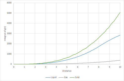
Figure 14: The Radial distribution against the distance of solid, liquid and gas	Figure 15: The integral of the RDF against the distance

2. Discuss qualitatively the differences between the three RDFs, and what this tells you about the structure of the system in each phase.

The radial distribution function, g(r) in a system of particles shows the probability of finding particles within a shell of distance r away from a reference atom.

In figure 14, at small distances, the RDF is zero for solid, liquid and gases due to the inter atomic repulsion at these distances.

Also, the solid has a large number of peaks due to long range order of the system. The fact that it has lots of peaks suggests the system has a large density.

Again, looking at figure 14, for gases and liquids the equilibrium RDF (where the line becomes horizontal) signifies the region where the probability of finding a particle from a reference point is the same. This would be when the particles are more or less equally distributed. The region between RDS = 0 and where equilibrium is reached, corresponds to when the particles are affected by the Lennard Jones potential and hence the probability varied slightly depending on whether the attractive or repulsive forces dominate. For liquids and gases there are very little peaks corresponding to short range order. The peaks are also smooth due to the molecular dynamics of the system.

Figure 15 shows the integration of g(r) against the distance. The integral of the RDF gives an idea of the average coordination number. Figure 15 shows that the coordination number of solids are greatest and the is lowest for gases. In reality coordination numbers are only significant in solids.

JC: The RDF is normalised so the number of peaks doesn't necessarily indicate the density of the system. The peaks indicate that the liquid has short range order, and the solid has long range order.

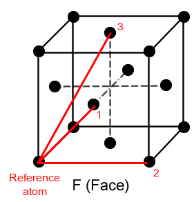
3. In the solid case, illustrate which lattice sites the first three peaks correspond to. What is the lattice spacing? What is the coordination number for each of the first three peaks?

molecule1
Figure 16

Figure 16 shows the lattice points that the distances of the first three peaks on the solid radial distribution function corresponds to.

	lattice point 1	lattice point 2	lattice point 3
Distance	1.025	1.475	1.825
Coordination number	12	6	24

The lattice spacing is the spacing between two lattices which is the distance between the reference atom and lattice point 2. This is 1.475 unit distance.

JC: Good idea to show the which atoms are responsible for the first three peaks on a diagram of an fcc lattice. Did you get the coordination numbers from the integral of the RDF? You could have calculated the lattice parameter from each of the first three peaks and then calculated an average rather than just taking the value of the second peak.

Dynamic properties and the diffusion coefficient

In this section, we are going to characterise the diffusion coefficient to get an idea of how the atoms move about in the simulation.

1. Make a plot for each of your simulations, showing the mean squared displacement as a function of timestep. Are these as you would expect?

molecule1
Figure 17: A plot of the mean square displacement as a function of timestep of simulations

The mean squared displacement is a measure of the deviation time between the position of a particle and some reference position.

As the time progresses it is expected that the position of a particle and some reference position would increase as it diffuses. This explains why there is a positive correlating line for solids, liquids and gases in figure 17. The gradient of the line correponds to $\frac{\partial ⟨r^2\left(t\right)⟩}{\partial t}$. The equation $D=\frac{1}{6}\frac{\partial ⟨r^2\left(t\right)⟩}{\partial t}$ is then used to obtain the diffusion coefficient. The diffusion coefficient gives an indication of the diffusion mobility. It can be seen that the gradient of the lines and hence the diffusion coefficient changes with the trend D(solid) < D(Liquid) < D(Gas). This is the expected trend as gas particles have a greatest diffusion mobility as gas systems have the lowest density. On the contrary solids have the lowest diffusion mobility as the particles in solids are in a fixed lattice and hence shows very little to no diffusion.

2. Repeat this procedure for the MSD data that you were given from the one million atom simulations.

molecule1
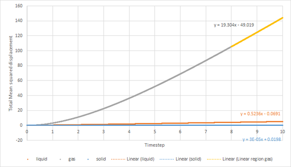Figure 18: A plot of the mean square displacement as a function of timestep of a million atoms

JC: Plot the different phases on separate plots so that they are easier to see. Do you know why the gas phase MSD begins as a curved line (ballistic motion)?

3. In the theoretical section at the beginning, the equation for the evolution of the position of a 1D harmonic oscillator as a function of time was given. Using this, evaluate the normalised velocity autocorrelation function for a 1D harmonic oscillator:

$C\left(\tau \right)=\frac{\underset{-\mathrm{\infty }}{\overset{\mathrm{\infty }}{\int }}v\left(t\right)v(t+\tau )\mathrm{d}t}{\underset{-\mathrm{\infty }}{\overset{\mathrm{\infty }}{\int }}{v}^2\left(t\right)\mathrm{d}t}1$ -(1)

From the 1D Harmonic Oscillator:

$x\left(t\right)=A\cos (\omega t+\varphi )$

$v\left(t\right)=\frac{\partial \left(x\left(t\right)\right)}{\partial t}=-A\omega \sin (\omega t+\varphi )$ -(2)

Substitute (2) into (1)

$C\left(\tau \right)=\frac{\underset{-\mathrm{\infty }}{\overset{\mathrm{\infty }}{\int }}A\omega \sin (\omega t+\varphi )\cdot A\omega \sin (\omega (t+\tau )+\varphi )\mathrm{d}t}{\underset{-\mathrm{\infty }}{\overset{\mathrm{\infty }}{\int }}{\sin }^2(\omega t+\varphi )\mathrm{d}t}$

$C\left(\tau \right)=\frac{\underset{-\mathrm{\infty }}{\overset{\mathrm{\infty }}{\int }}\sin (\omega t+\varphi )\cdot \sin (\omega t+\omega \tau +\varphi )\mathrm{d}t}{\underset{-\mathrm{\infty }}{\overset{\mathrm{\infty }}{\int }}{\sin }^2(\omega t+\varphi )\mathrm{d}t}$

Using $\sin (\alpha +\beta )=\sin \alpha \cos \beta +\sin \beta \cos \alpha ,$

$\sin (\omega t+\omega \tau +\varphi )=\sin (\omega t+\varphi +\omega \tau )=\sin (\omega t+\varphi )\cos \left(\omega \tau \right)+\sin \left(\omega \tau \right)\cos (\omega t+\varphi )$

$\therefore C\left(\tau \right)=\frac{\underset{-\mathrm{\infty }}{\overset{\mathrm{\infty }}{\int }}\sin (\omega t+\varphi )\cdot (\sin (\omega t+\varphi )\cos \left(\omega \tau \right)+\sin \left(\omega \tau \right)\cos (\omega t+\varphi ))\mathrm{d}t}{\underset{-\mathrm{\infty }}{\overset{\mathrm{\infty }}{\int }}{\sin }^2(\omega t+\varphi )\mathrm{d}t}$

$C\left(\tau \right)=\frac{\underset{-\mathrm{\infty }}{\overset{\mathrm{\infty }}{\int }}{\sin }^2(\omega t+\varphi )\cos \left(\omega \tau \right)+\underset{-\mathrm{\infty }}{\overset{\mathrm{\infty }}{\int }}\sin \left(\omega \tau \right)\cos (\omega t+\varphi )\sin (\omega t+\varphi )\mathrm{d}t}{\underset{-\mathrm{\infty }}{\overset{\mathrm{\infty }}{\int }}{\sin }^2(\omega t+\varphi )\mathrm{d}t}$

$C\left(\tau \right)=\cos \left(\omega \tau \right)+\frac{\underset{-\mathrm{\infty }}{\overset{\mathrm{\infty }}{\int }}\sin \left(\omega \tau \right)\cos (\omega t+\varphi )\sin (\omega t+\varphi )\mathrm{d}t}{\underset{-\mathrm{\infty }}{\overset{\mathrm{\infty }}{\int }}{\sin }^2(\omega t+\varphi )\mathrm{d}t}$

$C\left(\tau \right)=\cos \left(\omega \tau \right)+\frac{\underset{-\mathrm{\infty }}{\overset{\mathrm{\infty }}{\int }}\sin \left(\omega \tau \right)\cos (\omega t+\varphi )\mathrm{d}t}{\underset{-\mathrm{\infty }}{\overset{\mathrm{\infty }}{\int }}\sin (\omega t+\varphi )\mathrm{d}t}$

$\sin (x)=\text{odd function}$ $\cos (x)=\text{even function}$

$\text{odd function}\times \text{even function}=\text{odd function}$

$\sin (x)\cos (x)=\text{odd function}$

$\therefore \underset{-\mathrm{\infty }}{\overset{\mathrm{\infty }}{\int }}\cos (\omega t+\varphi )\sin (\omega t+\varphi )=0$

$\therefore \frac{\underset{-\mathrm{\infty }}{\overset{\mathrm{\infty }}{\int }}\sin \left(\omega \tau \right)\cos (\omega t+\varphi )\sin (\omega t+\varphi )\mathrm{d}t}{\underset{-\mathrm{\infty }}{\overset{\mathrm{\infty }}{\int }}{\sin }^2(\omega t+\varphi )\mathrm{d}t}=0$

$\therefore C\left(\tau \right)=\cos \left(\omega \tau \right)$

JC: Good, clear derivation and well spotted that you can avoid the integration by noticing that the integrand is an odd function.

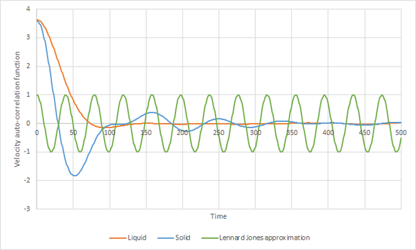
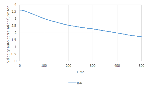
4. On the same graph, with x range 0 to 500, plot $C\left(\tau \right)$ with $\omega =1/2\pi$ and the VACFs from your liquid and solid simulations. What do the minima in the VACFs for the liquid and solid system represent? Discuss the origin of the differences between the liquid and solid VACFs. The harmonic oscillator VACF is very different to the Lennard Jones solid and liquid. Why is this?

molecule1	molecule1
Figure 19	Figure 20

A single atom at time zero has a certain velocity. If the atoms in the system do not interact with each other, due to conservation of energy the atom would retain this velocity.Therefore without the interaction between atoms the graph would just show a horizontal line. In low density systems, like gases, where the interaction between the atoms are very small, we would expect a gradual decrease in velocity as shown in figure 20. In high density systems such as solids and liquids where the interaction and forces between the atoms are strong, the atoms seek locations where there is a balance between the repulsive and attractive forces, as this is where the atom is most energetically stable. In solids the locations of the atoms are very stable hence they do not move far from their position. The oscillations will oscillate back and forth, reversing their velocity at each end. This is where the approximated graph in figure 19 comes from. The oscillations in the solid are damped by the perturbative forces acting on the atoms. Liquids are similar to solids however as the atoms in liquids are more diffusive the oscillatory motion is rapidly damped. The minima on the solid and the liquid represent the highest velocity of the damped oscillation in the opposite direction to where it started. The harmonic oscillator VACF is very different from the Lennard Jones solid and liquid because the harmonic oscillator assumes that there is a conservation in energy whereas the lennard Jones solid and liquid takes into account the interactions between the particles.

JC: What are the perturbative forces that cause the solid VACF to decay? The shape of the VACF is not due to conservation of energy, it is due to collisions between particles which randomise the velocities and cause the VACF to decorrelate. There are no collisions in the harmonic oscillator so no collisions.

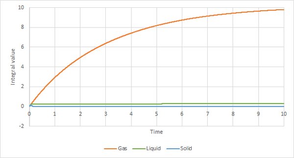
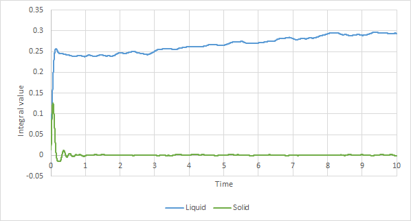
5. Use the trapezium rule to approximate the integral under the velocity autocorrelation function for the solid, liquid, and gas, and use these values to estimate $D$ in each case. You should make a plot of the running integral in each case. Are they as you expect? Repeat this procedure for the VACF data that you were given from the one million atom simulations. What do you think is the largest source of error in your estimates of D from the VACF?

molecule1	molecule1
Figure 21: Integral of VACF against time	Figure 22: Integral of VACF against time for a million atoms

molecule1	molecule1
Figure 23: Integral of VACF against time of liquid and solid only	Figure 24: Integral of VACF against time for a million atoms of liq and solid only

Figures 23 and 24 is the integral value versus the time. It shows the cumulative integral value of the velocity auto-correlation function as the time increases. Figure 20 shows that there area under the curve decreases per timestep which explains why the integral value of the gas shown in figure 21 shows an increases and plateaus. The integral value of the solid is near to zero through the timesteps because the areas on positive and negative areas on figure 19 cancel out. For the liquid graph, the an sharp increase in the integral value at the start comes from the positive area under the graph at the start on figure 19.

The diffusion coefficients from the VACF graphs are calculated using the equaiton:

$D=\frac{1}{3}\underset{0}{\overset{\mathrm{\infty }}{\int }}\mathrm{d}\tau ⟨\mathbf{v}\left(0\right)\cdot \mathbf{v}\left(\tau \right)⟩$

molecule1
Figure 25: diffusion coefficient (units: area/time)

Figure 25 shows the calculated diffusion coefficients from the mean squared distance over time graph and the velocity auto-correlation function graph. Earlier it was estimated by looking at the gradients of figure 17 that the diffusion coefficients followed the trend D(solid) < D(Liquid) < D(Gas). This statement is reinforced by the diffusion coefficients in the table. The diffusion coefficients obtained using the velocity auto-correlation function gives larger values than those calculated using the mean squared distance. The largest error comes from the trapezium rule which over estimates the area under the curve.

JC: Again show the different phases on different plots. This approach to calculating the diffusion coefficient from the VACF is only valid if the integral has converged within the simulation time so this is another possible source of error.