Talk:Mod:MH2015LS

NJ: General comments: A great start, some lovely explanation of the concepts in the early part of the experiment. The end seems very rushed, so I assume you ran out of time, which is a shame.

Molecular Dynamics - Liquid Simulation

A third year computational chemistry exercise by Michael Howlett.

Harmonic Oscillator

TASK: Complete the three columns "ANALYTICAL", "ERROR" and "ENERGY" in the excel file provided.

File:X(t) graph.png

Position vs time elapsed

Energy vs time elapsed

Error vs time elapsed

A comparison of the classical harmonic oscillator with the velocity-Verlet method by modelling with a partially prepared data set. Basic graphical analysis of the trends and error have been conducted and presented below.

'ANALYTICAL' values for the position of a harmonic oscillator given by:

$x(t)=Acos(\omega t+\varphi )$

'ERROR' values are given by the modulus of the difference between the harmonic oscillator and velocity-Verlet results for position x(t):

$Error=|x_{HO}(t)-x_{VV}(t)|$

'ENERGY' values represent the total energy of the oscillator as calculated in the velocity-Verlet system by the sum of the potential and kinetic components:

$Energy=\frac{1}{2}(k{x}^2+m{v}^2)$

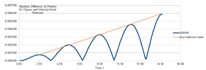
Graphical representation of these results are supplied by the thumbnails on the left.

In summary, there is only a very small deviation between the two methods according to the x(t) vs time graph. Additionally as can be seen, the total energy of the approximate velocity-Verlet system fluctuates about the constant average of the exact solution.

This is consistent with the conservation of energy that we expect for a real situation in which the energy is soley transferred between potential and kinetic forms.

Finally, the absolute error between the two models waxes and wanes through clear maxima with an overall trend of increasing as the simulation progresses.

TASK: For the default timestep value, 0.1, estimate the positions of the maxima in the ERROR column as a function of time. 

Classical harmonic oscillator / velocity-Verlet error maxima as a function of time:

Error maxima vs time elapsed

time	2.00	4.90	8.00	11.10	14.20
Error value /x10-3	0.758	2.00	3.30	4.60	5.91

 TASK: Experiment with different values of the timestep to discover the point at which the total energy change is = 1%. 
Why is it important to monitor the total energy of a physical system when modelling its behaviour numerically?

The limiting timestep to prevent >1% change in the total energy during the simulation is = 0.200 as shown by the inserted graph.

Percentage change in energy vs timestep value

timestep value	0.100	0.125	0.150	0.175	0.200	0.230
% change	0.25	0.39	0.56	0.77	1.00	1.27

It is important to monitor the total internal energy change throughout a simulation in order to assess how well the model meets the condition that energy must be conserved. In accordance with the Law of the Conservation of Energy, for an isolated simulated system, such as a box of simple particles, the total internal energy should remain constant to reflect that seen by experiment.

Any fluctuations seen are likely due to the approximations made in the computation and should be minimised in order to make the model more realistic. Such deviation from this physical law is a reflection upon the quality of the approximations made to simulate the system and thus measurements of this deviation can provide numerical information about the accuracy of the simulation.

Lennard-Jones Potential

TASK: For a single Lennard-Jones interaction,$\varphi (r)=4ϵ(\frac{{\sigma }^{12}}{r^{12}}-\frac{{\sigma }^6}{r^6})$, find the separation, $r_0$, at which the potential energy is zero. 

Typical Lennard-Jones potential

$\varphi (r)=4ϵ(\frac{{\sigma }^{12}}{r_0^{12}}-\frac{{\sigma }^6}{r_0^6})=0$

Therefore: $\frac{{\sigma }^{12}}{r_0^{12}}-\frac{{\sigma }^6}{r_0^6}=0$

$\frac{{\sigma }^{12}}{r_0^{12}}=\frac{{\sigma }^6}{r_0^6}$

$\frac{{\sigma }^{12}}{{\sigma }^6}=\frac{r_0^{12}}{r_0^6}={\sigma }^6=r_0^6$

It follows that: $\sigma =r_0$

What is the force at this separation? 

$F(r_0)=\frac{d\varphi (r_0)}{d{r}_0}=\frac{d(4ϵ({\sigma }^{12}{r}_0^{-12}-{\sigma }^6{r}_0^{-6})}{d{r}_0}$

From: $r_0=\sigma$, $F(r_0)=4ϵ(\frac{6}{r_0}-\frac{12}{r_0})$

$F(r_0)=\frac{-24ϵ}{r_0}$

NJ: The force is actually the negative of the derivative, but all correct otherwise. This is a net repulsive force as $r_0<r_{eq}$ which is a higher energy bond distance.

Find the equilibrium separation,$r_{eq}$ , and work out the well depth ($\varphi (r_{eq})$). 

$\frac{d\varphi (r_{eq})}{d{r}_{eq}}=\frac{d(4ϵ({\sigma }^{12}{r}_{eq}^{-12}-{\sigma }^6{r}_{eq}^{-6})}{d{r}_{eq}}=0$

$=4ϵ(6{\sigma }^6{r}_{eq}^{-7}-12{\sigma }^{12}{r}_{eq}^{-13})=0$

Therefore: $6{\sigma }^6{r}_{eq}^{-7}=12{\sigma }^{12}{r}_{eq}^{-13}$

$r_{eq}=\sigma \sqrt[6]{2}\approx 1.122\sigma$

Using the result that: $r_{eq}=\sigma \sqrt[6]{2}$

$\varphi (r_{eq})=4ϵ(\frac{{\sigma }^{12}}{r_{eq}^{12}}-\frac{{\sigma }^6}{r_{eq}^6})=4ϵ(\frac{{\sigma }^{12}}{{\left(\sigma \sqrt[6]{2}\right)}^{12}}-\frac{{\sigma }^6}{{\left(\sigma \sqrt[6]{2}\right)}^6})=4ϵ(\frac{{\sigma }^{12}}{{\sigma }^{12}{2}^2}-\frac{{\sigma }^6}{{\sigma }^{6}2})$

$=4ϵ(\frac{1}{4}-\frac{1}{2})=-ϵ$

Evaluate the integrals $\underset{a\sigma }{\overset{\mathrm{\infty }}{\int }}\varphi (r)dr$ for $a=2.0,2.5,3.0$ when $\sigma =ϵ=1.0$ .

$\underset{a\sigma }{\overset{\mathrm{\infty }}{\int }}\varphi (r)dr=[4ϵ\sigma (\frac{r^{-5}}{5}-\frac{r^{-11}}{11}){]}_{a\sigma }^{\mathrm{\infty }}$

Integral of Lennard-Jones potential

NJ: Lovely presentation of this.

TASK: The Lennard-Jones parameters for argon are $\sigma =0.34nm,ϵ/k_b=120K$If the LJ cutoff is $r^{*}=3.2$, what is it in real units? 

$r=r^{*}\sigma =3.2\times 0.34nm=1.088nm$

What is the well depth in kJ/mol? 

From the derivative of $\varphi (r)$ we know that for $r_{eq}$, the well depth is = $-ϵ$ Therefore for the magnitude of the argon well depth, find ε. From the argon Lennard-Jones parameters $ϵ=k_b\times 120=8.314\times 10^{-3}\times 120=9.98\times 10^{-1}kJ/mol$

What is the reduced temperature $T^{*}=1.5$ in real units?

$T=\frac{T^{*}ϵ}{k_b}=1.5\times 120=180K$

Simulation theory - additional exercises and questions

TASK: Estimate the number of water molecules in 1 mL of water under standard conditions. Estimate the volume of 1 mole of water molecules under standard conditions.

Density of pure water at 0°C $(STP)=0.999g/mL$, at 25°C $(SATP)=0.997g/mL$

STP: $Mr=18.015g/mol$ Therefore for $0.999/18.015=0.05545moles$ $0.05545\times 6.022\times 10^{23}=3.3394\times 10^{22}$ molecules of H2O.

SATP: $Mr=18.015g/mol$ Therefore for $0.997/18.015=0.05534moles$ $0.05534x6.022\times 10^{23}=3.3327\times 10^{22}$ molecules of H2O.

$10000/6.022\times 10^{23}=1.6606\times 10^{-21}moles$ $\times 18.015g/mol=2.9915\times 10^{-20}g$

$/0.999=2.9945\times 10^{-20}mL$

$/0.997=3.0005\times 10^{-20}mL$

Absolutely tiny fraction of 1 mL, i.e. an impossibly small volume for real world use.

TASK: Consider an atom at position  in a cubic simulation box which runs from  to  . In a single timestep, it moves along the vector  . At what point does it end up, after the periodic boundary conditions have been applied?.

Without periodic boundary conditions, a real atom in this scenario would end up at position vector [1.2, 1.1, 0.7] with respect to the origin in the starting box. However with the periodic boundary conditions applied in a simulation, the particle will 'reappear' at the opposite side of the box as it crosses the boundary into the adjacent simulated box. Therefore, traveling [0.7, 0.6, 0.2] from the middle of the original box, [0.5,0.5,0.5], the atom will end the timestep in position [0.2, 0.1, 0.7].

Periodic boundary diagram

Not only does this keep the number of atoms in the box constant but it enables us to build a better model of a macroscopic system. This is due to all the atoms being surrounded by a simulated environment 'infinitely' in all directions and they aren't faced with a sharp drop in potential or a vacuum on the exterior of the box.

TASK: Why do you think giving atoms random starting coordinates causes problems in simulations?

Were atoms to be too close to each other in their initial state then there is the possibility that this could lead to strong intermolecular interactions (due to the large dependency of the Lennard-Jones potential on distance r) and atom pairs could be formed at the equilibrium bond length. Taking this idea further, clusters of atoms could become strongly attracted to eachother and this behaviour wouldn’t accurately simulate the desired state. Alternatively of course, the other side of this is that atom pairs that were generated too close to each other, $r<r_{eq}$, could have a very high energy intial state in the simulation and could lead to eratic velocities and more collisions.

TASK: Satisfy yourself that this lattice spacing corresponds to a number density of lattice points of 0.8.

$lattice.point.density=\frac{(number.of.lattice.points.per.lattice\times total.number.of.lattices)}{(number.of.lattices.on.side.of.cube\times lattice.side.length{)}^3}$

$lattice.point.density=\frac{(1\times (10{)}^3)}{((10\times 1.07722{)}^3}=0.8$

Consider instead a face-centred cubic lattice with a lattice point number density of 1.2. What is the side length of the cubic unit cell?

For the 1.2 fcc density case:

$lattice.side.length=\frac{\sqrt[3]{{\frac{(lattice.point.density)}{(number.of.lattice.points.per.lattice\times total.number.of.lattices)}}^{-1}}}{(number.of.lattices.on.a.side.of.cube)}$

$lattice.side.length=\frac{\sqrt[3]{{\frac{(1.2)}{(4\times (10{)}^3)}}^{-1}}}{(10)}=1.49380$ ,

Confirmed by simulation of fcc lattice type.

As shown in diagram, with an atom at each lattice point, the inter-atom spacing is half that of the lattice unit cell side length. Lattice types and features

TASK: How many atoms would be created by the create_atoms command if you had defined the fcc lattice instead?

For a 10 x 10 x 10 cube of fcc lattices. Atom at every lattice point and 4 lattice points per fcc lattice. Therefore for the pre-set simulation box of 10 x 10 x 10 for a 0.8 lattice point density with a fcc system the number of atoms produced = 4000.

TASK: Using the LAMMPS manual, find the purpose of the following commands in the input script: 
mass 1 1.0
pair_style lj/cut 3.0
pair_coeff * * 1.0 1.0

• Gives the atom type (1) the mass of 1.0. There is only one atom type in these simulations.
• Instructs LAMMPS which method to use to calculate pairwise interactions between atoms. A cutoff distance for atom pairing is also defined, here as 3.0.
• Specifies the pairwise force field coefficients for the atom types.

NJ: What are the coefficients in this case?

TASK: Look at the lines below. What do you think the purpose of these is?

SPECIFY TIMESTEP
variable timestep equal 0.001
variable n_steps equal floor(100/${timestep})
variable n_steps equal floor(100/0.001)
timestep ${timestep}
timestep0.001
RUN SIMULATION
run ${n_steps}
run 100000 

On the second line,why not just write: 
timestep 0.001
run 100000 ?

Because it enables you to change a single line that specifies the value of the variable ‘timestep’ and the change will be propagated,including in equations, through the rest of the script without extra work.

NJ: This section makes sure that you always simulate the same time (nsteps*dt), no matter what timestep is chosen.

Equilibrium simulations

TASK: Given that we are specifying$x_i(0)$ and$v_i(0)$ , which integration algorithm are we going to use?

Velocity-Verlet Method

TASK: make plots of the energy, temperature, and pressure, against time for the 0.001 timestep experiment.

0.001 timestep whole simulation

Does the simulation reach equilibrium? How long does this take?

Initial equilibration of 0.001 timestep

The system does reach an equilibrium in which the temperature and pressure fluctuate about an average value. The total energy is, as expected, constant throughout. As shown by the plot the system reaches this average equilibrium state within 0.2 - 0.4 units time.

File:Energy vs time for all timesteps.png

Total energy vs time for all timesteps

Of the five timesteps that you used, which is the largest to give acceptable results? Which one of the five is a particularly bad choice? Why? Please see the thumbnail inserted for a large view of the energy profile of the 5 different timesteps. 0.0025 is a good one to choose. It can simulate 2.5x the actual time covered vs the 0.001 but with a very small change in the average energy value according to the graphs.

A bad choice would be a timestep as larger as 0.015 because it is not showing a constant energy which is a big indicator that it is simulating a real physical system poorly. Additionally, for simulations like these with a timestep of ~0.02 it has been observed that atoms are actually 'lost' from the box because the snapshots of what is happening are too far apart and an atom has crossed a periodic boundary twice and has been declared 'lost'. This is a big breakdown in the workings of the program but would be rectified by using a smaller timestep.

NJ: Very good

Running simulations under specific conditions

TASK: Choose 5 temperature and two pressures. This gives ten phase points — five temperatures at each pressure. Submit these ten jobs to the HPC portal.

TASK: We need to choose $\gamma$ so that the temperature is correct.

TASK: Solve these to determine $\gamma$.

$\frac{1}{2}\sum _i{m}_i{v}_i^2=\frac{3}{2}N{k}_{b}T\frac{1}{2}\sum _i{m}_i(\gamma v_i{)}^2=\frac{3}{2}N{k}_b\tau \frac{1}{2}\sum _i{m}_i(\gamma v_i{)}^2={\gamma }^2\frac{1}{2}\sum _i{m}_i{v}_i^2={\gamma }^2\frac{3}{2}N{k}_{b}T=\frac{3}{2}N{k}_b\tau \mathrm{\$}\gamma =\sqrt{\frac{\tau }{T}}$

TASK: Use the manual page to find out the importance of the three numbers 100 1000 100000.

How often will values of the temperature, etc., be sampled for the average? How many measurements contribute to the average? Looking to the following line, how much time will you simulate?

• Nevery = use input values every this many timesteps; every 100 timesteps = variables are sampled.
• Nrepeat = # of times to use input values for calculating averages
• Nfreq = calculate averages every this many timesteps; every 100000 timesteps = average calculated from sampled data i.e. once for simulation.

TASK: Plot the density as a function of temperature for both of the pressures that you simulated.Is your simulated density lower or higher? Justify this. Does the discrepancy increase or decrease with pressure?

Density vs Temperature graph with Ideal Gas Law plots and error bars]

Clearly from the graph the simulated density is higher than that calculated from the ideal gas law (approximately 3-times larger).The error values calculated during the simulation and plotted as error bars show that this discrepancy cannot simply be a case of error in the calculations as the difference is too large.

One plausible theory is that although a simple system only, the atoms in the box do not represent an ideal gas to a great extent. This would seem likely as there are pair interactions built into the simulation such that there are attractive (and repulsive) forces which could be more likely to bring the group of atoms together on the whole than if they were behaving as if without any intermolecular forces. This small amount of order provided by these forces could be enough to increase the density of the system above that of an ideal gas.

There seems to be little change to the density with increasing pressure and this could potentially support the idea of interactions establishing a stable level of order and increased density as the effects of pressure may be counteracted by a repulsive force between the atoms as they are squeezed into closer proximity.

NJ: This is very strange, the ideal gas law should give a higher density than the simulation. I suspect there is a problem with your ideal gas law curve. However, you've made a plausible explanation of the data you have. Why does the discrepancy change with temperature in the way that it does?

Calculating heat capacities using statistical physics

TASK: Plot heat capacity as a function of temperature for both of your densities. 

Is the trend the one you would expect? Attach an example of one of your input scripts to your report.

(Volume-normalised) Heat capacity vs Temperature for densities: 0.2 & 0.8

Trend for increasing temperature is in accordance with dependency of heat capacity on temperature at constant volume: $C_V=(\frac{\delta U}{\delta T}{)}_V$

NJ: This suggests that dU/dT = -T? What about the dependence with density?

File:Nvt script part 1.png

Adapted script for the calculation of the heat capacity of the systemPart 1 of 2

File:Nvt script part 2.png

Adapted script for the calculation of the heat capacity of the systemPart 2 of 2

Structural properties and the radial distribution function

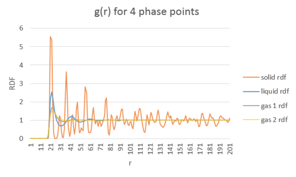
TASK: perform simulations of the Lennard-Jones system in the three phases. When each is complete, download the trajectory and calculate  and  . Plot the RDFs for the three systems on the same axes, and attach a copy to your report. 

Running integral of g(r)

File:Phase point chart.png

Phase point chart

Discuss qualitatively the differences between the three RDFs, and what this tells you about the structure of the system in each phase. In the solid case, illustrate which lattice sites the first three peaks correspond to. What is the lattice spacing? What is the coordination number for each of the first three peaks?

Dynamical properties and the diffusion coefficient

TASK: make a plot for each of your simulations (solid, liquid, and gas), showing the mean squared displacement (the "total" MSD) as a function of timestep. Are these as you would expect? Estimate  in each case. Be careful with the units! Repeat this procedure for the MSD data that you were given from the one million atom simulations.

File:Solid MSD 1M.png

Solid MSD 1M atoms

File:Liquid MSD 1M.png

Liquid MSD 1M atoms

File:Vapour MSD 1M.png

Vapour MSD 1M atoms

〈r^2 (t)〉=2dDt+C

NJ: Good to include this. What is the value of C?

(1/2d)* (∂〈r^2 (t)〉)/∂t = D

D = diffusion coefficient (Units: distance2/unit time), d = number of dimensions, C = constant (representing in the solid, the mean squared displacement of an atom in a crystalline fcc lattice at equilibrium) D = gradient /2d Own simulations: Ds = 3.82x10-8/ (2 X 3) = 6.367 x10-9 Dl = 5.09x10-1/ (2 X 3) = 8.483 x10-2 Dv = 9.41/ (2 X 3) = 1.568 Million atoms: Ds = 3.18x10-8/ (2 X 3) = 5.300 x10-9 Dl = 5.24x10-1/ (2 X 3) = 8.733 x10-2 Dv = 1.88x101/ (2 X 3) = 3.133

Diffusion coefficient is in this case unitless but not dimensionless (m^2/s) i.e length^2/time

NJ: Do these follow the trend you would expect?

At short times, the plot is not linear. This is because the the path a molecule takes will nearly be a straight line until it has a collision. Only when it starts the collision process will its path start to resemble brownian motion. NJ: Good. The curved section is called the "ballistic regime"

TASK: Evaluate the normalised velocity autocorrelation function for a 1D harmonic oscillator.

$x(t)=Acos(\omega t+\varphi )v(t)=\frac{d(x(t))}{dt}=A\omega sin(\omega t+\varphi )C(\tau )=\frac{\underset{-\mathrm{\infty }}{\overset{\mathrm{\infty }}{\int }}v(t)v(t+\tau )dt}{\underset{-\mathrm{\infty }}{\overset{\mathrm{\infty }}{\int }}{v}^2(t)dt}=\frac{\underset{-\mathrm{\infty }}{\overset{\mathrm{\infty }}{\int }}{A}^2{\omega }^{2}sin(\omega t+\varphi )sin(\omega (t+\tau )+\varphi )dt}{\underset{-\mathrm{\infty }}{\overset{\mathrm{\infty }}{\int }}{A}^2{\omega }^{2}si{n}^2(\omega t+\varphi )dt}=\frac{\underset{-\mathrm{\infty }}{\overset{\mathrm{\infty }}{\int }}sin(\omega t+\varphi )sin(\omega (t+\tau )+\varphi )dt}{\underset{-\mathrm{\infty }}{\overset{\mathrm{\infty }}{\int }}si{n}^2(\omega t+\varphi )dt}Sin(x+y)=sin(x)cos(y)+sin(y)cos(x)C(\tau )=\frac{\underset{-\mathrm{\infty }}{\overset{\mathrm{\infty }}{\int }}si{n}^2(\omega t+\varphi )cos(\omega \tau )+sin(\omega t+\varphi )sin(\omega \tau )cos(\omega t+\varphi )dt}{\underset{-\mathrm{\infty }}{\overset{\mathrm{\infty }}{\int }}si{n}^2(\omega t+\varphi )dt}=\frac{cos(\omega \tau )\underset{-\mathrm{\infty }}{\overset{\mathrm{\infty }}{\int }}si{n}^2(\omega t+\varphi )+sin(\omega \tau )\underset{-\mathrm{\infty }}{\overset{\mathrm{\infty }}{\int }}sin(\omega t+\varphi )cos(\omega t+\varphi )dt}{\underset{-\mathrm{\infty }}{\overset{\mathrm{\infty }}{\int }}si{n}^2(\omega t+\varphi )dt}=cos(\omega \tau )+\frac{sin(\omega \tau )\underset{-\mathrm{\infty }}{\overset{\mathrm{\infty }}{\int }}sin(\omega t+\varphi )cos(\omega t+\varphi )dt}{\underset{-\mathrm{\infty }}{\overset{\mathrm{\infty }}{\int }}si{n}^2(\omega t+\varphi )dt}=cos(\omega \tau )\underset{-\mathrm{\infty }}{\overset{\mathrm{\infty }}{\int }}sin(\omega t+\varphi )cos(\omega t+\varphi )dt=0\tau =0,C(\tau )=1\tau =\mathrm{\infty },C(\tau )=undefined$

This result is justified for all values of tau including infinity as the system is a harmonic oscillator and therefore the correlation of the variables with that system will fluctuate.

NJ: I'm not sure what you mean here.

Plot of the VACFs from the liquid and solid simulations.

VACF for simulated solid and liquids and for mathematically derived harmonic oscillator

TASK: Use the trapezium rule to approximate the integral under the velocity autocorrelation function for the solid, liquid, and gas, and use these values to estimate D in each case. You should make a plot of the running integral in each case.

File:Running integral S+L+V.png

Running integral - Solid, Liquid and Vapour

File:Running integral no vapour.png

Running integral - Solid and Liquid

Repeat this procedure for the VACF data that you were given from the one million atom simulations.

File:Running integral 1M atoms.png

Running integral 1M atoms - Solid, Liquid, Vapour

File:Running integral 1M atoms no vapour.png

Running integral 1M atoms - Solid and Liquid

What do you think is the largest source of error in your estimates of D from the VACF?

The largest source of error appears to be the use of the trapezium rule. Although generally a useful approximation it's nature lends it to either over or under estimate the function, giving a less accuract integral.

NJ: How do the VACF results compare with the MSD ones?