Talk:Mod:MDhz4813

JC: General comments: A lot of questions missing. You need to explain your results and what they tell you about your simulations. Make sure you understand the background theory behind each task.

1.Introduction

Liquids are very important in our life. This is not only because liquid is a state of matters, but also because many technologies processes, biological molecules molecules, membrane and ourselves process or live in liquid medium like water. Thus forces in such systems will determine and explain a lot of phenomenons and properties of everyday things. This is the reason why we need to study liquids at molecular level.

In recent years, a lot of accomplishments of molecular theories in liquids have been achieved. Because get exact solutions for Schrodinger equation of liquids are impossible, molecular approach become a utility way to analysis liquid. In the molecular approach, a molecule usually is modeled in its known properties ( like bond angles, charge distribution, etc.). Then a computer works out how a system composed of such molecules behaviors when the molecule in the system is allowed to interact with its neighboring molecules with interaction potential like the Lennard-Jones potential. Such computer simulation provides a useful insight to properties of liquid at molecular level.

There are two famous techniques of computer simulations. One is the Monte Carlo (MC) and the other one is Molecular Dynamics (MD). In this experiment, we will focus on the MD method. In this method, computer will calculate force on the molecule by solving the Newton equations. This force determined movement of the molecule. Then computer will work out such forces of all molecules we are interested (often said molecules in the box). Trajectories of those molecules also can be achieved as function of time. In equilibrium, the MC and MD methods will get the same final results about position. However, the MD method can provide information about how the molecule moves. Since the MD method also can be used to non-equilibrium and time-dependent system.

2.Theory

2.1 Velocity-Verlet algorithm

By using the velocity-Verlet algorithm, the behavior of a classical harmonic oscillator will be calculated.

Figure 1: Position as a function of time as timesept equal 0.1.

Figure 2: Energy as a function of time as timesept equal 0.1.

Figure 3: Error as a function of time as timesept equal 0.1.

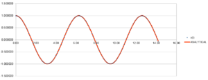
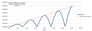
Position is a periodical function (shown in figure 1) with time with 6.4 second as period time and amplitude is positive and negative 1. The energy of this oscillator (shown in figure 2)is also a periodical function with time. The period time is 3.2 seconds and amplitude is 5E-001. Error (shown in figure 3)between analysis value and value got by velocity-Verlet algorithm shows periodical property with time. the period is 3.2 seconds and amplitude increases with time.

JC: For what value of timestep is the fluctuation in energy about 1 percent?

2.2 Atomic Forces

When we calculate force between molecules, we assume that Lennard-Jones potential is associated with this force.

For a single pair potential, $\varphi \left(r\right)=4ϵ(\frac{{\sigma }^{12}}{r^{12}}-\frac{{\sigma }^6}{r^6})$ where σ is a constant, ϵ is vacuum permittivity constant and r is distance between two interacted particle.

When the potential is zero, r=σ. Force between those two molecules, F=-dφ/dr. When r=σ, F=-24ϵ/σ=-24.

If such pair molecules reaches their equilibrium position, pair potential reach its minimum point.Which means dφ/dr=0. The separation distance at this state,

req=(2σ)^(1/6)=2^(1/6)=1.12 At this separated distance, pair potential φ(r)=4ϵ(σ^12/4 -σ^6/2 )=-2.

$\underset{2\sigma }{\overset{\mathrm{\infty }}{\int }}\varphi \left(r\right)\mathrm{d}r$=-0.004

$\underset{2.5\sigma }{\overset{\mathrm{\infty }}{\int }}\varphi \left(r\right)\mathrm{d}r$=-0.0009

$\underset{3\sigma }{\overset{\mathrm{\infty }}{\int }}\varphi \left(r\right)\mathrm{d}r$=-0.00026

JC: Maths correct, but show your working.

The Lennard-Jones potential is a special case of the Mie potential (in 1903), which is $\varphi \left(r\right)=\frac{A}{r^m}-\frac{B}{r^n}$. The Mie potential is the first time that a formula included both a repulsive term and an attractive term. The negative term in both equation is an expression of attractive term and positive term is associated with repulsive term. In the Lennard-Jones potential, when the separated distance is too small, the potential is positive, which means the repulsive force is dominant. Before reach the equilibrium distance, potential decreases with increasing distance. this means the attractive interaction contribute increasing effect with increasing distance. After the equilibrium distance, the potential decreases and goes to 0 at infinity. This shows when two molecules are far away to each other, the force between them is too small to ignore it. This conclusion also can be shown quantitively by three integrals we calculated above. Those integrals mean total potential from a typical distance to infinity. When the distance increase, the potential become smaller. If r=3σ, potential can be ignore. Thus when we calculate a total force of a molecule in a liquid, interaction of this molecule with distant molecules can be neglect.

2.3 Periodic Boundary Condition

In our simulations, we need to assume number of molecules before calculation. In 1 ml of water in standard condition, there are 6.02*10^23 water molecules and its volume is 18 mL. If there are 10000 water molecules, 2.998E-19 mL.

2.4 Reduced Units

When *r=3.2, $$\begin{gathered} \sigma =0.34\mathrm{n}\mathrm{m},r=1.088nm.<math>ϵ \\ / \\ {k}_B=120\mathrm{K} \end{gathered}$$, ϵ=1.66E-21. The Lennard-Jones potential φ=0.037$$\begin{gathered} {\mathrm{k}\mathrm{J} \\ \mathrm{m}\mathrm{o}\mathrm{l}}^{-1} \end{gathered}$$. T=180K

JC: Show your working. Question on periodic boundary conditions missing. 1 ml of water at standard conditions is not 1 mole so there are not 6x10²3 molecules in it. You need to work out the value of epsilon in kJmol-1.

3. Equilibration

3.1 Creating the simulation box

When we simulate a liquid, we generate a random position for each atom. However, in reality, atom cannot be actually random position. Mention for The Lennard-Jones potential, there two part in the equation with different signs. One of those two term associated with attractive potential and the other one terms by repulsive potential. When distance between two atom is small, pair potential between them is positive. Which means the repulsive potential is dominant. This is un-favourite. Thus that pair distance is too small is forbidden in real case.

JC: Why can't atoms be generated at random conditions, what is the problem with high repulsive forces?

Thus, atoms are always going to assume to be lattice point. From our input and output files, they show that the number density is 0.8 and lattice distance is 1.07722. The number of density should be number of lattice divides lattice volume. In this case, it is simple cubic, thus lattice number in one lattice unite is 1. Thus the number of density equal 0.8. For a face-centred cubic lattice, the lattice number in one lattice unit should equal 4 and the number density is 1.2. Thus the lattice distance is 1.7.

JC: This is very unclear. Show your working.

If we create_atoms in Face-centred lattice, there will be 1000 unit lattice. In face-centred lattice, each unit lattice has 4 lattice points. Thus, there will be 4000 atoms.

3.2 Setting the properties of atoms

mass 1 1.0
pair_style lj/cut 3.0
pair_coeff * * 1.0 1.0

The meaning of this input script is the mass of atom 1 is 1.0; cutoff Lennard-Jones potential with no Coulomb with pair distance 3.0 and there are only one type of atom, and pair coefficient of this atom to all other atom is 1.0.

In computer simulation, if initial condition of positions and velocities are known, we can use Velocity-Verlet algorithm.

JC: What are the pair coefficients for the Lennard-Jones potential?

3.3 Running the simulation

### SPECIFY TIMESTEP ###
variable timestep equal 0.001
variable n_steps equal floor(100/${timestep})
variable n_steps equal floor(100/0.001)
timestep ${timestep}
timestep 0.001

### RUN SIMULATION ###
run ${n_steps}
run 100000

In our program, we need to write as the first one. Before we run simulation, we need to let LAMMPS know the the variable name. The $ followed by curly brackets tell LAMMPS the name. The variable name is the text inside the curly brackets. In second express, LAMMPS does not what variety is, thus it can run the simulation.

JC: This is not answering the question, why is it better to use variables?

3.4 Checking equilibrium

Figure 4: Figures of energy, temperature and pressure as function of time when timesept equal 0.001.

Figure 5: Figures of energy, temperature and pressure as function of time when timesept equal 0.0025.

Figure 6: Figures of energy, temperature and pressure as function of time when timesept equal 0.0075.

Figure 7: Figures of energy, temperature and pressure as function of time when timesept equal 0.01.

Figure 8: Figures of energy, temperature and pressure as function of time when timesept equal 0.015.

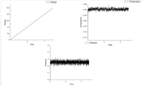
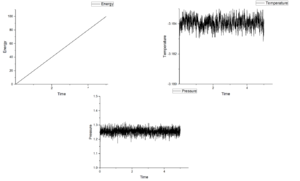
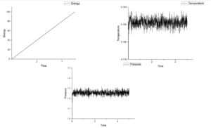
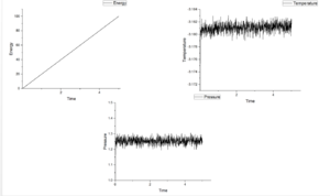
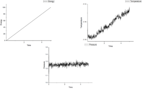
Figure 4-8 shows graph of energy, temperature and pressure as function of time under different timestep. According figures of energy, energy increases as growing time at those five timesteps. This means this system do not reach equilibrium. If it is under equilibrium, there will be a minimum value in energy. When timesteps increase from 0.001 to 0.15, the value of pressure fluctuate around 1.25 and the more smaller timestep the more noisy. Temperature should show the same tendency as pressure. However, when timestep is 0.015, temperature shows an increasing trend. For this reason, this measurement is the worst among five measurements.

JC: Plot the energy for each timestep on the same graph to compare the different timesteps. Which timestep did you choose?

4.Under specific conditions

1.Thermostats and Barostats $E_K=\frac{3}{2}N{k}_{B}T$

$\frac{1}{2}\sum _i{m}_i{v}_i^2=\frac{3}{2}N{k}_{B}T$ multiply every velocity $\gamma$

$\frac{1}{2}\sum _i{m}_i{\gamma }^2{v}_i^2=\frac{3}{2}N{k}_{B}T$

${\gamma }^2=\frac{3N{k}_{B}T}{\sum _i{m}_i{v}_i^2}$

JC: Simplify this further, the final answer should be gamma = squareroot(target temperature/current temperature).

2. The input script

100 is the Number of every, 1000 is the number of repeat, and 100000 is the Number of frequency arguments specify on what timesteps the input values will be used in order to contribute to the average.

Figure 9: Figures of density as function of temperature when pressure is 1.25 and timesept equal 0.01.

Figure 10: Figures of density as function of temperature when pressure is 1.75 and timesept equal 0.01.

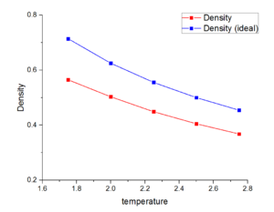
Figure 9 and 10 shows linear relationship between density and temperature at two different pressure. The density decrease when temperature increase. The line in red in both figure stand our stimulate value of density and red is ideal gas density calculated by ideal gas equation. Our stimulate value in both cases are smaller than ideal gas density. When pressure increase from 1.25 to 1.75, the density increases in theory. However, our stimulated value do not have obviously change. This is maybe because the different between two pressures is too small.

JC: The relationship between density and temperature is not linear (in ideal gas density = 1/T). Why is the ideal gas density higher than the simulation density?

5.Heat capacity

Figure 11.

Figure 12.

Figure 13: Figure of heat capacity as function of temperature under two different density.

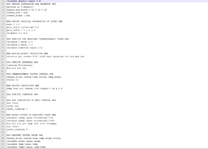
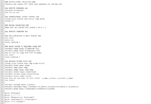
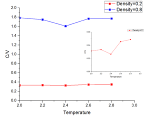
Figure 11 and 12 show part of script of heat capacity. Figure 13 shows heat capacity as function of temperature. When density increases, heat capacity also increase. In both density, heat capacity shows a minimum value at temperature equal 2.4.

JC: You need to explain the trends that you see in your results.

6.Structural properties and the radial distribution function

Figure 14: Figure of the radial distribution function as function of distance under there different states.

Figure 15: Figure shows integral of the radial distribution function as function of distance under there different states.

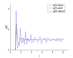
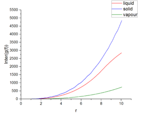
Figures 14 shows the relationship between the radical distribution function and distant under three different physical states. Those three functions reach the maximum values around one and function has the largest value at solid state. Around 2, distribution function of vapor reaches a stable value at about 1. Distribution function of solid and liquid fluctuate around 1. Figure 15 expresses the integral of radical distribution function under three different physical states. All of this function increase with distance. In solid state, this function grows most fastest, then liquid state and final vapour state.

JC: You haven't answered any of the questions in the task, why do the solid, liquid and gas RDFs look so different, what is the lattice parameter, how many first, second and third nearest neighbour atoms are there?

7. Dynamical properties and diffusion coefficient

Figure 15: Figure of the mean squared displacement as function of timestep under liquid state.

Figure 16: Figure of the mean squared displacement as function of timestep under solid state.

Figure 17: Figure of the mean squared displacement as function of timestep under vapour state.

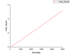
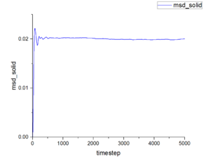
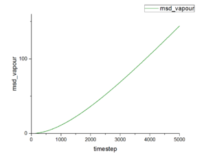
Figure 15-17 show the mean squared displacement as the function of timestep under three different physical states. The mean squared displacement of liquid and vapour increase with growth of timestep. However, the value at vapour state is much larger than that at liquid state. This function under solid state shows fluctuate when timestep is small and at stable value at rest of timestep and the smallest value among those three states. Conclusion according to those graphs suggests common result from our life. Particles in vapour can move the freest, then particles in liquid. Particles in solid have nearly fixed position-they only can vibration and rotation.

JC: You should have calculated a numerical value for the diffusion coefficient. What about the VACF?