JC: General comments: Great report with well thought out written answers showing a good understanding of the material. Try to make the layout clearer so that it is easier to see where you have answered each question and show your working for calculations. Also try to write a bit more concisely so that your arguements are clearer.

Molecular dynamics simulations of simple liquids

MISSION 1: Introduction to molecular dynamics simulation

OBJECTIVE A: Reconnaissance of errors in the velocity-Verlet algorithm simulation of a classical harmonic oscillator. No room for mistakes! Reduce change in energy below 1%.

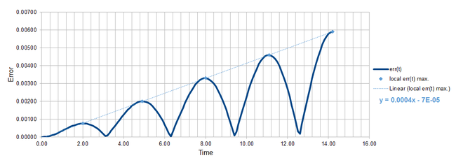
REPORT A: A file containing the velocity-Verlet (v-V) algorithm for a classical harmonic oscillator was provided to us at the start of the mission. This algorithm requires initial conditions for the position and the velocity, x(0) and v(0) respectively. The position at time t depends on the position one time step before x(t-dt) and the velocity half a time step before v(t-0.5dt). With this dependence, it was apparent that errors would tend to accumulate over the course of our simulations. First, we compared the errors in the position x_v(t) between solution from the v-V algorithm and the classical solution given in our case as x_c(t) = cos(t). The error was calculated as err(t) = |x_v(t)-x_c(t)| and the plot over the course of the simulation is shown in Figure 1.

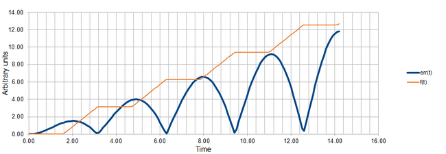
Next we aimed to find a function that would help us find the local maxima in the error err(t). At the maximum, the first derivative of err(t) with respect to t must be zero. Below is showed the function f(t) proposed to help us find the times at which the aforementioned condition is fulfilled.

$\frac{d e r r (t)}{d t} = \frac{d x_{v} (t)}{d t} - \frac{d x_{c} (t)}{d t} = 0 = v_{v} (t) + s i n (t) ⟹ proposed function: f (t) = t - a r c s i n (∣ v_{v} (t) ∣)$

Figure 2 shows in one plot the functions err(t) and f(t). The start- and end-points of the plateaus in the f(t) correspond well to the maxima in err(t) near the end of the simulation. As we mentioned above, the algorithm accumulates the errors over time, thus near the beginning of the simulation, there is a strong disagreement between the actual positions of the maxima in err(t) and the positions predicted by our function. Once enough errors have accumulated, the maxima in error start to behave more regularly and appear always when the absolute value of velocity v_v(t) reaches maximum. The light blue line in Figure 1 represents the empirical trend in the values of the local maxima from which the cumulative property of the errors is apparent as the error maxima clearly increase in value linearly with time.

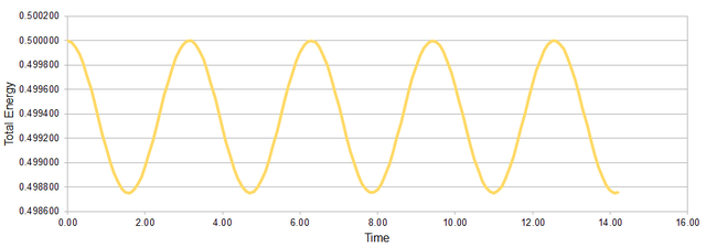
Figure 1 - The change in absolute value of error in position between the v-V algorithm and classical solution for classical harmonic oscillator over the course of the simulation. The linear trend in local maxima of the error is shown.	Figure 2 - Plot showing relation between functions err(t) and f(t).

Having examined the error in the position, we then looked at the change of the total energy in our v-V algorithm simulation of classical harmonic oscillator. Monitoring the total energy in simulations of systems and making sure that it does not change significantly throughout the simulation is a good way of making sure that our simulation is not horribly useless. The total energy in the classical harmonic oscillator system is calculated as:

$E = \frac{1}{2} m v^{2} + \frac{1}{2} k x^{2}$

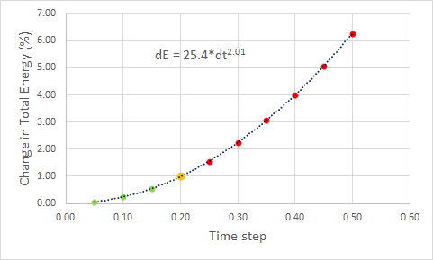
Figure 3 illustrates the oscillatory behaviour of the total energy in our system with simulation time step 0.1 as a cos(2t): period 1π. The minima in the total energy in the system correspond to points where the displacement x is zero (the displacement follows cos(t): period 2π and reaches zero every π time units). The change in the total energy dE depends on the time step used in the simulations - this relationship is shown in Figure 4 where we find dE to roughly increase with second power of dt. The breaking point in dt after which the change in energy surpasses the bearable 1% limit is found to be 0.2.

Figure 3 - The fluctuation in the total energy in the v-V algorithm simulation of classical harmonic oscillator with time step 0.1.	Figure 4 - The dependence of the total energy fluctuation dE on the time step dt.

JC: Good choice of timestep. Why did you try to fit a function to the error to find the maxima and what do you mean by "the maximum in error starts to behave more regularly"? Why does the error oscillate?

OBJECTIVE B: Acting forces, cubes and reduced units. Unlock your potential!

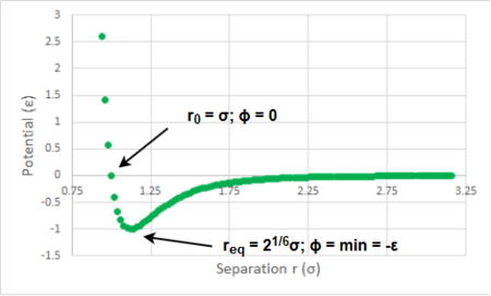
**Figure 5** - Plot of Lenard-Jones potential

REPORT B: We move from a classical harmonic oscillator towards an anharmonic one - i.e. at infinite separation r the interatomic interactions are zero and at smaller than the equilibrium separation r_eq the repulsive forces grow faster than in the harmonic oscillator. The anharmonic oscillator is described by the Lennard-Jones potential given as (plot in Figure 5):

$ϕ (r) = 4 ϵ (\frac{σ^{12}}{r^{12}} - \frac{σ^{6}}{r^{6}})$

There exist two interesting separations. The first one r₀ is a separation at which the potential is zero. By simple arithmetics, r₀ is found to be r₀ = σ : sigma is the interatomic separation at which the potential ϕ(r) is zero. The second interesting separation is the equilibrium one r_eq at which the attractive and repulsive forces cancel out - at this point the potential is at its minimum (as shown in Figure 5) and thus r_eq can be found by equating the first derivative of ϕ(r) to zero. For a single Lenard-Jones interaction, the first derivative is equal to the total force acting on the particle. We found successfully the separation r_eq (force is zero there) for which we also calculated the potential well depth to be -ε : epsilon is thus the potential minimum on the Lenard-Jones potential plot. At the zero-potential separation r₀ we calculated the acting force and found it to be a repulsive force which agrees with our hypothesis that when the particles are too close they will repel.

$F_{i} = \frac{d ϕ (r)}{d r} = 4 ϵ (- 12 \frac{σ^{12}}{r^{13}} + 6 \frac{σ^{6}}{r^{7}})$

$⟹ at equilibrium separation: 4 ϵ (- 12 \frac{σ^{12}}{r^{13}} + 6 \frac{σ^{6}}{r^{7}}) = 0 ⟹ r = 2^{1 / 6} σ ⟹ ϕ (r) = - ϵ$

$⟹ at zero-potential separation: r = σ ⟹ F_{i} = - 24 \frac{ϵ}{σ} ⟹ repulsive force$

So far, we only considered the interactions between two particles. However, we want to model a liquid system probably with more than two particles. In such case, the potential energy of one particle is then the sum of all the interactions with the remaining particles - but to model such a system a lot of computational power is required. For example, if we wanted to model 1 mL of water which contains 3.35*10²² particles, we would then need to calculate that many interactions for every particle in the system. We instead try to simplify the system to save the power. We can limit ourselves to a smaller volumes and thus smaller numbers of particles - e.g. 10000 water particles under standard conditions occupy volume of 2.99*10^-19 mL - corresponding to a cube with a edge length of 669 nm. Or, fortunately, the strength of the interatomic interactions decays strongly with distance. Thus, it is reasonable to disregard any interactions with particles that are further than certain separation limit. To find this limiting separation, we evaluate the integrals of the potential from 2σ, 2.5σ and 3σ to infinity and compare them to the integral from r_eq to infinity. The obtained values are shown in Table 1. We see that at the 3σ separation the value of the integral is less than 1% of the integral value at the equilibrium separation and thus it seems reasonable to only consider the interactions with particles within this separation.

**Table 1** - Results of the integration of ϕ(r) from a starting separation to infinity with respect to r with ε=σ=1
Starting separation	Integral value
r_eq	-0.3469
2σ	-0.0258
2.5σ	-0.0082
3σ	-0.0033

Life (i.e. simulations of liquids) can be further simplified by introducing boundary conditions and using reduced units. With the boundary conditions, we simulate a cube containing particles and we make sure that the number of particles in the cube remains constant by making sure that if a particle leaves the cube through one face, it immediately reenters the cube from the opposite face. For instance, if we have an atom at position (0.5, 0.5, 0.5) in a cubic box running from (0, 0, 0) to (1, 1, 1) and this atom moves along the (0.7, 0.6, 0.2) vector, instead of ending up at position (1.2, 1.1, 0.7) which is outside the box it will end up at position (0.2, 0.1, 0.7).

With regard to the reduced units, if we consider a Lenard-Jones potential for argon with σ=0.34 nm and ε/k_b=120 K, instead of writing writing the cutoff separation as 1.088 nm we can instead express it in the reduced units as 3.2, or instead of writing temperature as 180 K we can express it in the reduced units as 1.5, and instead of writing the potential well depth as 0.997 kJ*mol^-1 we can express it in the reduced units as simply 1.

JC: All calculations correct, but show your working and would be clearer not to include your answers in a paragraph of text.

THIS IS THE END OF MISSION 1

REWARD 1: Two different approaches to introduction to liquid simulations: theory-first vs experiment-first.

MISSION 2: Equilibration

OBJECTIVE A: Understand the input script!

REPORT A: At the beginning of the simulation we arrange the particles of the modelled liquid into a highly ordered crystalline arrangement (e.g. simple cubic) - this, of course, does not correspond to the more disordered state of molecules in a real liquid but the simulation moves quickly towards more reasonable arrangement (example of 'how fast' discussed later below). We use this starting arrangement instead of a random initial arrangement to avoid problems that could arise from generating some particles too close together - as we saw previously with the Lenard-Jones potential the repulsive forces rise rapidly with decreasing separation (once below r_eq) and since these forces affect the velocities of our particles and since we use the velocity-Verlet algorithm (we specify initial position and initial velocity of each of the simulated particles) which bases the calculation of velocities and positions on the velocities in the previous time-steps - these unnaturally high repulsive forces at the beginning of the simulation would cause our simulation to diverge (example shown later) unless we would choose really small time step which is much more computationally demanding than to start from the ordered arrangement.

In our first simulations we use simple cubic lattice as the starting point with a number density 0.8. The density multiplied by the volume of the unit cell must equal 1 for sc lattice - one lattice point per unit cell. In a face-centred cubic lattice there are 4 lattice points per unit cell. The side-lengths of a cubic cell for a sc lattice with density 0.8 and fcc lattice with density 1.2 follow (n = number of lattice points per unit cell, a = side length of a unit cell, ρ = number density) ρ*a³=n and are equal to 1.07722 and 1.49380, respectively.

Once we have chosen the lattice type and specified the number density, we can then create a box containing e.g. 10x10x10=1000 unit cells - such box will contain 1000 atoms for sc and 4000 atoms for fcc.

At the beginning of each input script, we usually define any quantities (which we could consider changing later) as variables and use the variable down the script instead of using the hard number - this allows us to change all mentions of time-step in the script from 0.001 to 0.002 at once rather than having to go through the whole script and changing it several times.

Some important commands to consider:

mass 1 1.0 - sets the mass for atoms of type 1 to be 1.0.

pair_style lj/cut 3.0 - specifies that we use cutoff Lennard-Jones potential with no Coulomb as the pair potential used by LAMMPS with cutoff separation of 3 in reduced units.

pair_coeff * * 1.0 1.0 - sets the coefficients sigma and epsilon in the L-J potential to be equal to 1.0 for all (*) atom types.

JC: Good.

OBJECTIVE B: Choose wisely the time-step! You should not rush but don't be late either.

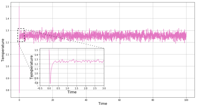
REPORT B: We use our input script to create a box with the simulated particles which have well defined initial position. The script also assigns particles random initial velocities in such a way that the mean square velocity remains constant and equal to value based on the fixed initial conditions. Every particle thus has well-defined x(0) and v(0) and the v-V algorithm can be applied on the system. Our script records the total energy, temperature and pressure throughout the simulation, and plots of these quantities for the simulation with time-step = 0.001 are shown in Figures 6-8, respectively. As we predicted above, with this relatively short time-step, the system equilibrates quickly from the high-energy initial state to the ground state within t = 0.5. The equilibration is observed in all 3 quantities, and once the equilibrium is reached these quantities continue to fluctuate around the equilibrium values within reasonably small range.

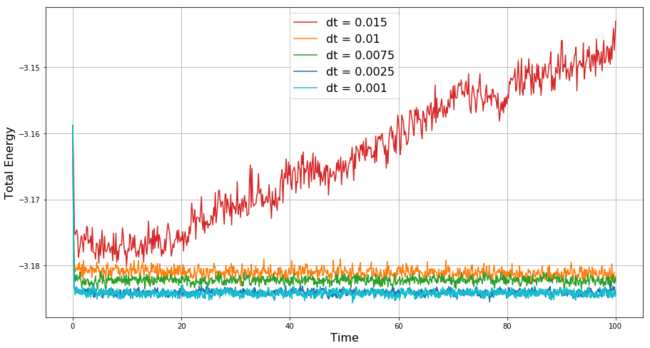
The simulation with the time-step 0.001 equilibrates successfully, but ideally we would like to obtain the same result with longer time-step, i.e. running less simulation points for a given time length of the simulation. A comparison in changes of total energy throughout 5 simulations with different time steps is shown in Figure 9. The simulation with the longest time-step = 0.015 is the only one that does not converge - it diverges because the time-step is too long to react accurately to the changes in the measured quantities and as we mentioned above the v-V algorithm tends to accumulate errors throughout the simulation, thus with the too long time-step during the most turbulent time in our simulation (i.e. the beginning) a significant error is accumulated within the first few steps and this makes it impossible for the simulation to converge to the correct values.

With the shorter time-steps 0.01 and 0.0075 we see that the simulation converges but not at the correct value obtained with time-step 0.001. This is again the result of the errors accumulated within the few initial steps of the simulation. Finally, the simulation with dt = 0.0025 not only converges but even converges to the same (i.e. well within acceptable limits) equilibrium value as the simulation with the shortest dt. Therefore, dt = 0.0025 is the optimal time-step for our simulation (from the 5 tested ones) and chosen to be used in the subsequent simulations.

Figure 6 - Change in Total Energy throughout the simulation with time-step = 0.001.	Figure 7 - Change in Temperature throughout the simulation with time-step = 0.001.
Figure 8 - Change in Pressure throughout the simulation with time-step = 0.001.	Figure 9 - Comparison of changes in Total Energy throughout simulations with different time-steps.

JC: Good choice of timestep and explanation.

THIS IS THE END OF MISSION 2

REWARD 2: Example of a liquid system with diverging total energy.

MISSION 3: Running simulations under specific conditions

OBJECTIVE: Find your balance! There is no pressure but try to run simulations at specified temperatures and pressures.

REPORT : Previous simulations were run in the microcanonical ensemble. We now move towards the canonical ensemble for which we specify in our script the temperature and pressure at which we want our simulation to be conducted. This more closely corresponds to a laboratory situation where we e.g. work at atmospheric pressure and control/keep fixed the reaction temperature.

Over the course of the simulation, the simulation has to try to keep the system temperature (and pressure) around the initially specified target. To do so, the simulation uses the equipartition theorem for the kinetic energy of the particles in our system which follows (as we have 3 degrees of translational freedom):

$E_{k} = \frac{1}{2} \sum_{i}^{} m_{i} v_{i}^{2} = \frac{3}{2} N k_{B} T (1)$

If the target temperature is T_t then the actual temperature at a given point in the simulation T can be either lower or higher, thus to get closer to the target temperature the simulation introduces a constant factor γ by which it multiplies the velocity of every particle, the γ for every step is determined as follows:

$\frac{1}{2} \sum_{i}^{} m_{i} (γ v_{i})^{2} = \frac{3}{2} N k_{B} T_{t} ⟹ (gamma independent of i) ⟹ \frac{1}{2} γ^{2} \sum_{i}^{} m_{i} v_{i}^{2} = \frac{3}{2} N k_{B} T_{t}$

⟹ (substitute from equation (1)) ⟹ γ^{2} \frac{3}{2} N k_{B} T = \frac{3}{2} N k_{B} T_{t} ⟹ γ^{2} = \frac{T_{t}}{T} ⟹ γ = \sqrt{\frac{T_{t}}{T}}

**Figure 10** - Change in density with temperature at constant pressure. Comparison between the simulation and ideal gas behaviour.

JC: Correct.

The simulation takes the square root of the ratio between the target temperature and temperature at a given step and uses this factor on the subsequent step. We can record the average temperature in our system by introducing the command: fix aves all ave/time 100 1000 100000 v_temp which says to record temperature once every 100 time-steps, to calculate the average out of 1000 inputs and to calculate the averages every 100000 time-steps. Thus if we run 100000 time-steps the average temperature will be recorded once at the end of our simulation from 1000 temperatures recorded every 100 time-steps.

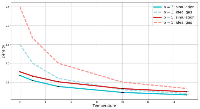
In this section, we use the script to record the average temperature, pressure, and density (and the corresponding errors for each of them) in simulations of 10 systems (5 dif. temperatures and 2 pressures). We compare the change in density with respect to temperature between the two pressures and between the behaviour expected for an ideal gas at these pressures. The plot of this dependence is shown in Figure 10 - the error bars representing the errors in both temperature and density are included and even though the errors in temperature start to become more apparent as the temperature increases, the errors in density remain negligible. Several observations can be obtained from Figure 10.

Firstly, at a given temperature, the fluid with higher pressure has higher density and these densities decay with increasing temperature when keeping the pressure constant. This is exactly what we should observe.

Secondly, we compare the simulated data for the fluid at 2 different pressures with the behaviour of an ideal gas in reduced units governed by:

$ρ = \frac{N}{V} = \frac{p}{T}$

At low temperatures, where the fluid is the most dense for a given pressure, we observe strong disagreement between the ideal gas and our simulated fluid. The density of the ideal gas is much higher and the discrepancy is stronger at the higher pressure. This is again exactly as we would expect. The ideal gas approximation assumes that there are no interactions between the particles apart from the perfectly elastic collisions, i.e. instead of having potential curve as the Lenard-Jones one (Mission 1 - Figure 5) we instead have hard spheres between which the potential remains zero going from infinite separation and then the potential shoots up to infinity once the spheres touch - this means that in ideal gas the particles do not repel each other and thus at a given temperature the ideal gas must be more dense in order to achieve the same pressure as a non-ideal fluid at the same temperature. The discrepancy is strongest at the lowest temperature and the higher pressure since under those conditions the particles in the non-ideal system are forced to interact with each other the most.

Lastly, as the temperature increases, in order to keep the pressure constant the density has to decrease, and as the density decreases - the average interatomic distances increase and the particles interact less which leads to a more ideal behaviour of the non-ideal system and to a better agreement between the simulation and the ideal gas.

JC: The particles in the ideal gas are not hard spheres - they have no volume and no interactions, otherwise the explanation is correct. Don't plot straight lines between the data points for the ideal gas as this is a bit misleading since we know that the ideal gas law doesn't follow this line.

THIS IS THE END OF MISSION 3

REWARD 3: You have reached middle of this project. If you are marking it while sitting down, reward your future self by standing up and stretching a bit.

MISSION 4: Calculating heat capacities using statistical physics

**Figure 11** - Change in heat capacity over volume with temperature for systems with fixed density.

OBJECTIVE: Do finally something sort of on your own! Write a script to study heat capacity of a simulated system.

REPORT : In this section, we made a script that calculates variance in energy and uses this to calculate heat capacity based on an equation that was provided to us. Our script works in NVT ensemble and we record C_V at 5 different temperatures for 2 systems with fixed density at 0.2 and 0.8 respectively. The results are shown in Figure 11. According to the phase diagram for Lennard-Jones system^[1], at these densities and pressures we are dealing with a super-critical fluid. There are two observations to be noted.

Firstly, the heat capacity over volume is lower for the system with lower density (unit cell volume = 5.000). This is exactly what we expect from the eqquipartition theorem which states that the heat capacity of a group of particles is directly proportional to the degrees of freedom and to the number of particles ( for 3 degrees of freedom and N particles: $C_{V} = \frac{3}{2} k_{B} N$ ). Thus, if we are comparing heat capacities between two equal volumes (i.e. alternative way of saying heat capacity over volume) it is clear that the system with higher density (unit cell volume = 1.250) and therefore with higher number of particles in a given volume must have higher heat capacity.

The second observed trend is the decrease in heat capacity with temperature. From our five data point, it appears to decrease linearly but that is not an expected behaviour (some form of exponential decay would be expected) and is probably just result of small number of data points within small range of temperature values. Regardless of the actual shape of the trend, the trend itself is what is interesting - i.e. the decrease in heat capacity with temperature. We saw an example of decrease in heat capacity during our Statistical Thermodynamics lectures. If we have a two level system, at low temperatures most particles are in the ground state and thus the system has high ability to accommodate additional energy. However, as temperature goes to infinity the two energy levels become almost equally populated and thus to follow Boltzmann distribution - it becomes increasingly harder to excite a particle from the ground state and therefore heat capacity decreases. If we now return to our system, the particles in our system accommodate energy by increasing their kinetic energy and thus their velocity.

Thus, the heat capacity depends on the ability of our particles to accommodate increase in velocity. Now the initial constraint of our system comes into play, i.e. the fact that the density is fixed. With increase in velocity, in order to keep density constant, we have to increase the pressure. As we increase the velocity, the collisions become more frequent and the relative volume occupied by our particles increases and the interatomic volume decreases - with increasing temperature the system becomes more restrained as the pressure increases and the space where a single particle can move decreases - it becomes increasingly more difficult to keep the density constant as the temperature increases. From this hypothesis, we would expect for the heat capacity to decrease with steeper slope for the system with higher density - and that is exactly what we observe the heat capacity per volume decreases in the higher-density system with slope = -0.047 and with slope = -0.039 in the lower-density system. There are certainly other competing factors affecting the heat capacity in our case, but based on agreement between the proposed hypothesis and the observed behavior it seem that the decrease in the relative freedom of the system with temperature is the deciding factor.

JC: Good suggestion. Both the kinetic and potential energy of the particles in the simulation increases when energy is put into the system and remember that these simulations are classical so there are no discrete energy levels. More frequent collisions do not increase the volume occupied by each particle.

An example of an input script used to record the heat capacities is shown below:

### DEFINE SIMULATION BOX GEOMETRY ###

variable density equal 0.2

lattice sc ${density}

region box block 0 15 0 15 0 15

create_box 1 box

create_atoms 1 box

### DEFINE PHYSICAL PROPERTIES OF ATOMS ###

mass 1 1.0

pair_style lj/cut/opt 3.0

pair_coeff 1 1 1.0 1.0

neighbor 2.0 bin

### SPECIFY THE REQUIRED THERMODYNAMIC STATE ###

variable T equal 2.2

variable timestep equal 0.0025

### ASSIGN ATOMIC VELOCITIES ###

velocity all create ${T} 12345 dist gaussian rot yes mom yes

### SPECIFY ENSEMBLE ###

timestep ${timestep}

fix nve all nve

### THERMODYNAMIC OUTPUT CONTROL ###

thermo_style custom time etotal temp press

thermo 10

### RECORD TRAJECTORY ###

dump traj all custom 1000 output-1 id x y z

### RUN SIMULATION TO MELT CRYSTAL ###

run 10000

unfix nve

reset_timestep 0

### BRING SYSTEM TO REQUIRED STATE ###

variable tdamp equal ${timestep}*100

variable pdamp equal ${timestep}*1000

fix nvt all nvt temp ${T} ${T} ${tdamp}

run 10000

reset_timestep 0

unfix nvt

fix nve all nve

### MEASURE SYSTEM STATE ###

thermo_style custom step etotal temp press density atoms

variable temp equal temp

variable temp2 equal temp*temp

variable Natm2 equal atoms*atoms

variable energ equal etotal

variable energ2 equal etotal*etotal

fix aves all ave/time 100 1000 100000 v_temp v_energ v_energ2

run 100000

variable avetemp equal f_aves[1]

variable varenerg equal (f_aves[3]-f_aves[2]*f_aves[2])

variable heatcap equal ${Natm2}*${varenerg}/${temp2}

print "Temperature: ${avetemp}"

print "Heat capacity: ${heatcap}"

THIS IS THE END OF MISSION 4

REWARD 4: There is no reward 4 but you are allowed to return to one of the Rewards 1-3.

MISSION 5: Structural properties and the radial distribution function

OBJECTIVE: Interatomic Affairs. If you can predict quite well atom arrangement even far away from the capital atom, that is a solid result.

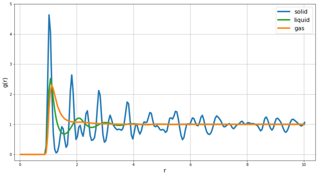
REPORT : In this section we look at the Radial Distribution Function (RDF) of a solid, liquid and gas phases in Lennard-Jones system. The RDF g(r) represents the probability of finding an atoms at a given distance r from the central atom. By integrating g(r) from zero to r we can calculate the number of particles that are located within the distance r from the central atom. At very small r values g(r) is zero as at this distance the particles would be too close to each other and the repulsive forces would be extremely high. Figure 12 shows the comparison of RDFs at T = 1.2 for gas (density = 0.07), liquid (density = 0.8) and solid (density = 1.2).

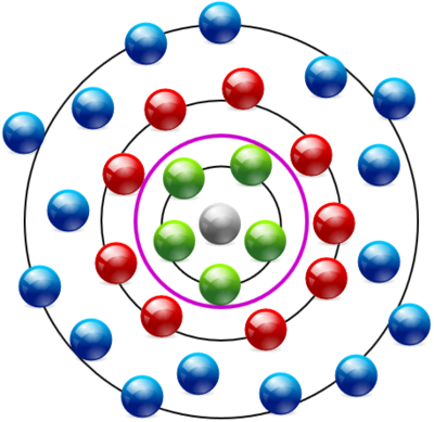
In the case of gas, we see a single peak and then the RDF decays to 1 - this shows us that in gas phase only the position of the nearest particles is affected by the central atom and there is no long distance order within the system. In the case of liquid, we observe 3-4 detectable peaks - this means the interactions between particles in the liquid phase are effective over longer distances - in our case there is detectable effect of the central atom on the particles within 3-4 interatomic distance - another aspect of the liquid RDF is the presence of parts of RDF that are below 1 - we have our central particle and then there are particles (green particles in Figure 14) that are likely to be found around r = 1.1 this then makes it unlikely for particles to be found at r = 1.5 (purple line Figure 14) as at this distance particles would strongly repel with the particles at r = 1.1 - then there is again region of increased likelihood (red particles in Figure 14) but the effects decay within 3-4 distances after which the relatively fast movement of particles in liquid phase averages out any effect of the central atom on the relative structure at these larger distances (blue particles in Figure 14).

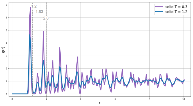
In the case of solid, the particles are fixed in crystalline lattice and cannot move around like they did in gas and liquid - this significantly increases the ability to predict the likelihood of finding particles even at large distances - the factor that slowly averages the RDF to zero at large distance in solids is the vibrational motion - thus we would expect to observe better resolution of the RDF at lower temperatures where the vibrational energy of the system is lower - this is exactly what is observed in Figure 13 which shows comparison of RDF of solid at 2 different temperatures - the better resolution (sharper peaks) is apparent for the system with T = 0.3. In our input script we set up the lattice as face-centered cubic, we now compare data obtained from the RDF with the expected ordering in fcc lattice. We integrated the RDF from zero to the 3 values highlighted in Figure 13 - i.e. the r values corresponding to the minima after each of the first 3 peaks.

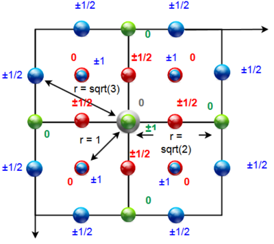
For integration up to the end of the first peak (r = 1.2), we get a value of 12.4 which correspond well to the expected coordination number in fcc lattice for the 12 nearest neighbors - the 12 red spheres shown in Figure 15. When integrating up to the end of the second peak (r = 1.67), we get a value of 18.0 which corresponds to the expected coordination number for the sum of the nearest neighbors (red spheres) and the new 6 next-nearest neighbors (green spheres in Figure 15). The ratio between the r values of the first two peaks is also in good agreement with expected 1 vs 2^0.5. The inter-layer distance can be calculated as a height in trigonal pyramid with edge-length equal to the distance between the nearest neighbors which is in our case 1.05 and thus the lattice spacing is 0.70.

The r value of the third peak is again at expected position 3^0.5 which corresponds to the distance of blue spheres in Figure 15 from the central grey one. There are 24 spheres of the blue type and thus we would expect the coordination number to be 18+24=42. However, by integrating the RDF up to to the end of the third peak (r = 2.0) we obtain value of only 28 - thus there is a strong disagreement between our predicted result and the obtained value - which is in strong contrast with the good agreement for the first two peaks. However, the overall expected trend - alternating peaks corresponding to the face-centred particles (higherpeak) and the corner-based particles (smaller peak) is apparent over large distances from the central particle.

Figure 12 - RDFs for gas, liquid and solid phases in Lennard Jones system.	Figure 13 - Comparison of RDF of Lennard-Jones solid at different temperatures.
Figure 14 - Ordering of particles in liquid phase.	Figure 15 - Lattice plan for the solid with fcc lattice.

JC: Nice idea to look at the effect of temperature on the solid phase RDF. Good diagram of the fcc lattice to show which atoms are responsible for which peaks, but the lattice parameter is the length of the unit cell, it should be about 1.5 for your simulations, not 0.7. Show a plot of the integral of the RDF, it should show 42 for the integral up to the third peak, are you sure you were looking at the value of r corresponding to the third peak?

THIS IS THE END OF MISSION 5

REWARD 5: We are out of ideas, just have a snack or something.

MISSION 6: Dynamical properties and the diffusion coefficient

OBJECTIVE: Examine diffusion-related aspects of the simulations and finally finish the project.

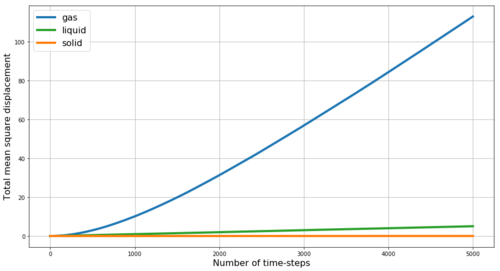
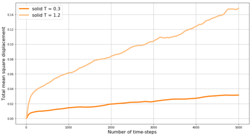
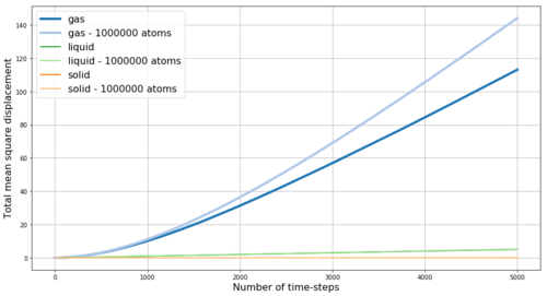
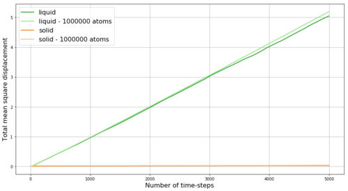
REPORT : Fist we look at the mean square displacement (MSD) for the gas, liquid and solid phases simulated in Mission 5. MSD is a measure of the extent of random motion - at constant temperature and thus with constant mean square velocities in our system we expect MSD to increase linearly. Also, we expect the slope to be steepest for gas and to be almost zero for the solid - as gas particles have the highest velocity while the solid particles are mostly fixed in the crystalline lattice. The obtained results are shown in Figure 16 - and the expected behavior is observed. Within the very first few steps (apparent in Figure 17) it takes some time for the linear trend to start, thus when obtaining the slope from linear fit, these points are excluded. By multiplying the slope of MSD by $\frac{1}{6}$ and by dividing by the value of time-step in reduced units (0.002) we obtain the diffusion coefficients D for our phases as follows: D(gas) = 2 m²s^-1, D(liquid) = 0.085 m²s^-1, D(solid) = 4.1*10^-4 m²s^-1. Here the small diffusivity of solid is even more apparent. However, the diffusion factor is temperature dependent as shown in Figure 17 by the comparison of the MSD for solid at two different temperatures - by increasing the temperature from 0.3 to 1.2 (i.e. 4-times) the diffusion coefficient of the solid increases 4.7-times to 1.93*10^-3 m²s^-1 - this trend is expected as with increasing temperature the energy in the system increases and makes it more likely for the particles to diffuse even in the solid phase. Density is expected to have opposite effect.

JC: The units are not m2s-1 unless the units of sigma are in metres. Why does the gas phase MSD begin as a curved line (ballistic motion)? The solid phase MSD seems to increase over time, is this what you'd expect for a solid? Have you started from an fcc or sc solid here?

Figures 18 and 19 show a comparison between MSDs from our simulation and from simulation with much larger number of particles. The overall trend between different phases is the same. The difference between the curves can be explained by the effect of different simulation temperatures or densities.

Figure 16 - Total mean square displacement for Lennard-Jones gas, solid and liquid.	Figure 17 - Comparison in total mean square displacement of solid at different temperatures.
Figure 18 - Comparison of the MSD from our simulations with MSDs from simulations of 1000000 atoms.	Figure 19 - Comparison of the MSD from our simulations with MSDs from simulations of 1000000 atoms.

Next, we evaluate the velocity autocorrection function (VACF) for our three phases as this can also be used to calculate the diffusion coefficient. We first find the solution of the VACF for the classical harmonic oscillator discussed in Mission 1.

$classical harmonic oscillator: x (t) = A c o s (ω t + ϕ) ⟹ v (t) = \frac{d x (t)}{d t} = - A ω s i n (ω t + ϕ)$

$normalised velocity autocorrelation function for a 1D harmonic oscillator: C (τ) = \frac{\int_{- \infty}^{\infty} v (t) v (t + τ) d t}{\int_{- \infty}^{\infty} v^{2} (t) d t} = \frac{\int_{- \infty}^{\infty} A^{2} ω^{2} s i n (ω t + ϕ) s i n (ω (t + τ) + ϕ) d t}{\int_{- \infty}^{\infty} A^{2} ω^{2} (s i n (ω t + ϕ))^{2} d t}$

$cross-out constants: \frac{\int_{- \infty}^{\infty} s i n (ω t + ϕ) s i n (ω (t + τ) + ϕ) d t}{\int_{- \infty}^{\infty} (s i n (ω t + ϕ))^{2} d t} = \frac{\int_{- \infty}^{\infty} s i n (ω t + ϕ) s i n (ω t + ϕ + ω τ) d t}{\int_{- \infty}^{\infty} (s i n (ω t + ϕ))^{2} d t}$

$use: s i n (a + b) = s i n (a) c o s (b) + c o s (a) s i n (b) and take out constant terms: \frac{\int_{- \infty}^{\infty} s i n (ω t + ϕ) s i n (ω t + ϕ) c o s (ω τ) + s i n (ω t + ϕ) c o s (ω t + ϕ) s i n (ω τ) d t}{\int_{- \infty}^{\infty} (s i n (ω t + ϕ))^{2} d t} = c o s (ω τ) \frac{\int_{- \infty}^{\infty} s i n (ω t + ϕ) s i n (ω t + ϕ) d t}{\int_{- \infty}^{\infty} (s i n (ω t + ϕ))^{2} d t} + s i n (ω τ) \frac{\int_{- \infty}^{\infty} s i n (ω t + ϕ) c o s (ω t + ϕ) d t}{\int_{- \infty}^{\infty} (s i n (ω t + ϕ))^{2} d t}$ $c o s (ω τ) \frac{\int_{- \infty}^{\infty} (s i n (ω t + ϕ))^{2} d t}{\int_{- \infty}^{\infty} (s i n (ω t + ϕ))^{2} d t} + s i n (ω τ) \frac{\int_{- \infty}^{\infty} s i n (ω t + ϕ) c o s (ω t + ϕ) d t}{\int_{- \infty}^{\infty} (s i n (ω t + ϕ))^{2} d t}$

In the left fraction we now have the same function in nominator and denominator which are both divergent in exactly the same way as they are the same function and we can write:

$c o s (ω τ) + s i n (ω τ) \frac{\int_{- \infty}^{\infty} s i n (ω t + ϕ) c o s (ω t + ϕ) d t}{\int_{- \infty}^{\infty} (s i n (ω t + ϕ))^{2} d t}$

For the remaining fraction, in nominator we use the identity: $c o s (a) s i n (a) = \frac{1}{2} (s i n (2 a))$ and in denominator we use: $(s i n (a))^{2} = 1 - (c o s (a))^{2} = (c o s (a))^{2} - c o s (2 a) = \frac{1}{2} (1 - c o s (2 a))$ . Thus:

$c o s (ω τ) + s i n (ω τ) \frac{\int_{- \infty}^{\infty} c o s (2 (ω t + ϕ)) d t}{\int_{- \infty}^{\infty} \frac{1}{2} (1 - c o s (2 (ω t + ϕ) d t} = c o s (ω τ) + s i n (ω τ) \frac{{[- \frac{c o s (2 (ω t + ϕ))}{4 ω}]}_{- \infty}^{\infty}}{{[\frac{2 (ω t + ϕ) - s i n (2 (ω t + ϕ))}{4 ω}]}_{- \infty}^{\infty}}$

We can write:

$C (τ) = c o s (ω τ) + s i n (ω τ) {[\frac{- \frac{c o s (2 (ω t + ϕ))}{4 ω}}{\frac{2 (ω t + ϕ) - s i n (2 (ω t + ϕ))}{4 ω}}]}_{- \infty}^{\infty} = c o s (ω τ) + s i n (ω τ) {[\frac{- c o s (2 (ω t + ϕ))}{2 (ω t + ϕ) - s i n (2 (ω t + ϕ))}]}_{- \infty}^{\infty}$

Now we evaluate the limits: $\lim_{t \to \infty} \frac{- c o s (2 (ω t + ϕ))}{2 (ω t + ϕ) - s i n (2 (ω t + ϕ))}$ and $\lim_{t \to - \infty} \frac{- c o s (2 (ω t + ϕ))}{2 (ω t + ϕ) - s i n (2 (ω t + ϕ))}$ . And since the range of values for both sine and cosine is between -1 and +1 along the whole t-axis - these limits tend to zero as t goes to ± $\infty$ due to the part $2 (ω t + ϕ)$ which approaches ± $\infty$ and is in denominator. Thus:

C (τ) = c o s (ω τ) + s i n (ω τ) * 0 = c o s (ω τ)

**Figure 20** - VACF for Lennard-Jones liquid and solid compared to VACF of classical harmonic oscillator.

JC: This derivation can be simplified by noticing that sin(x)*cos(x) is an odd function and so its integral with limits which are symmetric about zero, is zero.

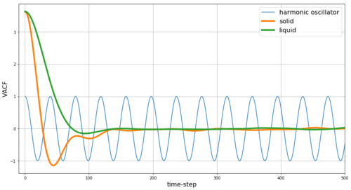
The VACF describes the dependence of the velocity after several time-steps on the initial velocity. Thus, in classical harmonic oscillator the above-obtained harmonic result is expected - i.e. if we start with some initial velocity at some initial displacement then we expect for the particle in the classical harmonic oscillator to have the same-in-value-but-opposite-in-direction velocity after $\frac{π}{ω}$ time-steps have passed which correspond to the minima in the VACF plot. However, in the cases of Lennard-Jones solids and liquids which instead follow the potential curve shown in Figure 5, we expect a damped oscillator behaviour instead. Further, we would expect the dampening to be weaker in the solid phase as the solid phase with the crystalline lattice more closely resembles the classical harmonic oscillator.

Our simulation data shown in Figure 20 agree with these predictions. Stronger dampening is observed for liquid phase compared to solid phase. In gas phase (not shown in our figures) the dampening is above the critical limit and thus only exponential decay without any harmonic behaviour is observed for the VACF of gas phase.

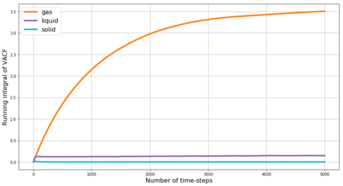
The diffusion coefficient can be obtained by integrating the VACF from zero to infinity with respect to time-step and dividing by 3. We use the trapezium rule to approximate the integrals under the VACFs for the gas, liquid and solid phases - the plot of the running integral is shown in Figure 21. However, as we only run 5000 time-steps instead of infinity, the running integral does not reach full plateau especially in case of the gas phase and this is a significant source or error in our estimate of D from VACF. The running integral is highest for gas phase and lowest for solid phase which agrees with the expected diffusions coefficients as discussed above. From VACF, we obtain the diffusion coefficients D for our phases as follows: D(gas) = 1.16 m²s^-1, D(liquid) = 0.05 m²s^-1, D(solid) = 3.7*10^-4 m²s^-1- compare with results from MSD: D(gas) = 2 m²s^-1, D(liquid) = 0.085 m²s^-1, D(solid) = 4.1*10^-4 m²s^-1. The results are relatively close in values and the best agreement is observed for the solid phases - i.e. the most ordered system. The value obtained from the VACF for gas is quite lower which agrees with our proposed source of error - i.e. the fact that the running integral under VACF does not have time to reach plateau (and thus higher values of D) within the 5000 simulated time-steps - by running longer simulations the diffusion coefficients from the two methods could be expected to converge at the same value. Figure 22 shows the running integrals also for the simulations with much larger number of atoms - and as in case of MSD the values reached by these simulations are higher that those reached with our simulated smaller number of particles - which we again attribute to higher temperature or lower density in the more-particle simulation.

Figure 21 - Running integral under VACF of Lennard-Jones gas, liquid and solid.	Figure 22 - Running integral under VACF of Lennard-Jones gas, liquid and solid - comparison of simulation with higher number of particles.

JC: Collision between particles randomise the particle velocities and cause the VACFs to decay, there are no collisions in the harmonic oscillator. Plot the integrals on separate graphs as it is hard to see the results for the solid and liquid.

THIS IS THE END OF MISSION 6

REWARD 6: You got through the whole thing - that's a reward by itself. Congratulation!

REFERENCES

↑ Hansen, Jean-Pierre P., and Loup Verlet. "Phase Transitions of the Lennard-Jones System." Physical Review 184, no. 1 (1969): 151-61.

[1] Hansen, Jean-Pierre P., and Loup Verlet. "Phase Transitions of the Lennard-Jones System." Physical Review 184, no. 1 (1969): 151-61.

[1]