Talk:Mod:Liquid simulations

JC: General commentsː Some good answers, but also some graphs and parts of questions are missing. Make sure you answer the questions in full before adding extra results and focus on making sure that your written explanations are clear.

Introduction to molecular dynamics simulation

Verlet algorithm for the 1D harmonic oscillator

Figure1: Error maxima as a function of time

Figure2: Total energy as a function of time

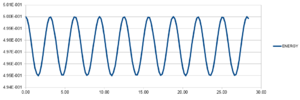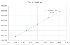
Fig. 1 shows the energy error maxima in time for a timestep of 0.1. As one can see from the figure itself, all the maxima lie on a straight line. The particular line $y=4*10^{-7}x-7*10^{-5}$ gives a perfect fit. From a practical point of view, however, a timestep this small is not necessary. It is important to note that the total energy of a harmonic oscillator is constant in time, so a fluctuation of 1% is good enough for practical purposes. If the error is too large or, even worse, it does not converge, the simulation becomes unrealistic (useless). Different timesteps have been tried and 0.2 is the largest acceptable timestep. This is because it gives a 1% maximum error in total energy, as fig. 2 shows.

JC: The fit isn't perfect if you look to more than 1 s.f. Good choice of timestep, how many others did you try?

Lennard-Jones potential

$\varphi (r)=4ϵ(\frac{{\sigma }^{12}}{r^{12}}-\frac{{\sigma }^6}{r^6})$

Separation $r_0$ at which the potential is zero is calculated as follows:

$\varphi (r_0)=0$

$\frac{{\sigma }^{12}}{r_0^{12}}-\frac{{\sigma }^6}{r_0^6}=0$

$\frac{{\sigma }^{12}}{r_0^{12}}=\frac{{\sigma }^6}{r_0^6}$

$\frac{{\sigma }^6}{r_0^6}=1$

$\frac{\sigma }{r_0}=1$

$r_0=\sigma$

This potential energy creates a conservative force field. Therefore, the force at any distance $r$ can be linked to the potential energy at the same distance by:

$F(r)=-\frac{d\varphi }{dr}$

$F(r)=4ϵ(-12\frac{{\sigma }^{12}}{r^{13}}+6\frac{{\sigma }^6}{r^7})$

$F(r)=24ϵ(\frac{{\sigma }^6}{r^7}-2\frac{{\sigma }^{12}}{r^{13}})$

At separation $\sigma$ this force is:

$F(\sigma )=24ϵ(\frac{{\sigma }^6}{{\sigma }^7}-2\frac{{\sigma }^{12}}{{\sigma }^{13}})$

$F(\sigma )=-24\frac{ϵ}{\sigma }$

The equilibrium position, $r_{eq}$, is the position where the force is zero. $F(r_{eq})=0$

Using the equation linking force to potential energy we obtain:

$24ϵ(\frac{{\sigma }^6}{r_{eq}^7}-2\frac{{\sigma }^{12}}{r_{eq}^{13}})=0$

$\frac{{\sigma }^6}{r_{eq}^7}=2\frac{{\sigma }^{12}}{r_{eq}^{13}}$

$1=2\frac{{\sigma }^6}{r_{eq}^6}$

$r_{eq}^6=2{\sigma }^6$

$r_{eq}=\sigma 2^{\frac{1}{6}}$

The well depth is given by the value of the potential at the equilibrium position, $\varphi (r_{eq})$.

$\varphi (r_{eq})=4ϵ(\frac{{\sigma }^{12}}{r_{eq}^{12}}-\frac{{\sigma }^6}{r_{eq}^6})$

$\varphi (r_{eq})=4ϵ(\frac{1}{4}-\frac{1}{2})$

$\varphi (r_{eq})=-ϵ$

Evaluating some relevant integrals:

$\underset{2\sigma }{\overset{\mathrm{\infty }}{\int }}\varphi (r)dr=4ϵ\underset{2\sigma }{\overset{\mathrm{\infty }}{\int }}(\frac{{\sigma }^{12}}{r^{12}}-\frac{{\sigma }^6}{r^6})=[4ϵ(-\frac{{\sigma }^{12}}{11r^{11}}+\frac{{\sigma }^6}{5r^5}){]}_{2\sigma }^{\mathrm{\infty }}=4ϵ\sigma (\frac{1}{11*2^{11}}-\frac{1}{5*2^5})=-0.0248ϵ\sigma$

$\underset{2.5\sigma }{\overset{\mathrm{\infty }}{\int }}\varphi (r)dr=[4ϵ(-\frac{{\sigma }^{12}}{11r^{11}}+\frac{{\sigma }^6}{5r^5}){]}_{2.5\sigma }^{\mathrm{\infty }}=4ϵ\sigma (\frac{1}{11*2.5^{11}}-\frac{1}{5*2.5^5})=-0.008ϵ\sigma$

$\underset{3\sigma }{\overset{\mathrm{\infty }}{\int }}\varphi (r)dr=[4ϵ(-\frac{{\sigma }^{12}}{11r^{11}}+\frac{{\sigma }^6}{5r^5}){]}_{3\sigma }^{\mathrm{\infty }}=4ϵ\sigma (\frac{1}{11*3^{11}}-\frac{1}{5*3^5})=-0.0032ϵ\sigma$

For $ϵ=\sigma =1.0$ the integrals become -0.0248, -0.008 and -0.0032 respectively.

JC: All maths correct and clearly laid out.

Water volume

Under standard conditions the density of water is $\rho =1\frac{g}{ml}$.

The volume of N=10000 molecules can be estimated as follows: The number of moles is

$n=\frac{N}{N_A}$

The mass is $m=n{\mu }_{water}$

$m=\frac{N{\mu }_{water}}{N_A}$

And finally, the volume can be written as $V=\frac{m}{\rho }$

$V=\frac{N{\mu }_{water}}{N_A\rho }$

$V=\frac{10000*18}{6.022*10^{23}*1}=3*10^{-19}ml$

JC: Correct, how many water molecules are there in 1 ml of water?

Moving a particle along a vector

The new position of the particle that is located initially at $r_0=(0.5,0.5,0.5)$ and moves along the vector $v=(0.7,0.6,0.2)$ can be calculated by adding these two vectors (component by component). The only problem is that the box has finite dimensions (1x1x1) and each time the particle leaves the box it reenters through the opposite face. In other words, each time a coordinate reaches the value of 1, it resets to 0 and the particle keeps moving until reaching the final position. Therefore, if the addition of the components produces a number that is larger than 1 we have to subtract 1 an integer number of times.

In this particular case, the coordinates become:

$x=0.5+0.7-1=0.2$

$y=0.5+0.6-1=0.1$

$z=0.5+0.2=0.7$

So the final position is:

$r=(0.2,0.1,0.7)$

Reduced units

$r^{*}=\frac{r}{\sigma }$

$r=r^{*}\sigma$

If $r^{*}=3.2$ then $r=3.2*0.34=1.088nm$

The well depth $ϵ$ in real units is $ϵ=120*1.38*10^{-23}=1.656*10^{-21}J$ In $\frac{kJ}{mol}$ the well depth becomes $ϵ=1.656*10^{-21}*10^{-3}*6.022*10^{23}=0.997\frac{kJ}{mol}$

$T^{*}=\frac{k_{B}T}{ϵ}$

$T=\frac{ϵT^{*}}{k_B}$

If $T^{*}=1.5$ then $T=120*1.5=180K$

JC: Correct.

Equilibration

Giving atoms a randomly distributed positions can lead to them being positioned very close to each other in the beginning, at distances much smaller than the equilibrium distance of the Lennard-Jones potential. Consequently, they will repel violently and pick up incredible speeds, something which will make simulating a liquid impossible.

JC: High repulsion forces can make the simulation unstable and cause it to crash.

Number density of lattice points

A simple cubic lattice having a lattice constant $a=1.07722$ in reduced units can have its number density of lattice points calculated as follows:

$$\begin{gathered} \rho =\frac{no \\ of \\ lattice \\ points}{V} \end{gathered}$$

A simple cubic lattice has 1 lattice point and a volume $V=a^3$.

$\rho =\frac{1}{a^3}$

$\rho =0.8$

For a face centered cubic lattice the only difference is the number of lattice points, which is 4. $$\begin{gathered} a=\sqrt[3]{\frac{no \\ oflattice \\ points}{\rho }} \end{gathered}$$

$a=\sqrt[3]{\frac{4}{1.2}}=1.49380$

For an fcc the number of atoms created will be 4 times larger than for an sc, because an fcc has 4 lattice points, while an sc has only 1. Therefore, the command create_atoms would generate 4000 atoms.

The purpose of the commands

mass 1 1.0
pair_style lj/cut 3.0
pair_coeff * * 1.0 1.0

is to define the mass of the atoms (in this case 1.0), to set the Lennard-Jones cutoff value (here at 3.0 in reduced units) and to define the Lennard-Jones potential parameters (\sigma and \epsilon, both set to 1.0). The Lennard-Jones cutoff value is the distance beyond which the potential is considered to be 0.

Next, the velocity Verlet algorithm is going to be used for the simulation, because it can take the initial velocity as an input.

JC: Correct, why is a cutoff used for this potential?

Running the simulation

The purpose of the second line from the following piece of code

### SPECIFY TIMESTEP ###
variable timestep equal 0.001
variable n_steps equal floor(100/${timestep})
variable n_steps equal floor(100/0.001)
timestep ${timestep}
timestep 0.001

### RUN SIMULATION ###
run ${n_steps}
run 100000

is to define timestep as a variable that can be used anywhere in the code. Therefore, if the timestep needs to be changed for a particular simulation, the value would only need to be changed ones, not everywhere in the code.

Figure 3: Energy as a function of time

Figure 4: Temperature as a function of time

Figure 5: Pressure as a function of time

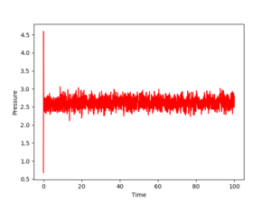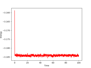
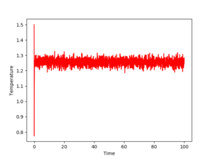
Figs. 3,4 and 5 show the evolution of the energy, temperature and pressure of the system for a timestep of 0.001. As one can see, all three parameters converge. Even if they fluctuate, these fluctuations give numbers that average to a constant value. Also, the equilibration is very quick, as the time needed for these quantities to stabilize is almost nonexistent (roughly 1 unit). This means the chosen timestep is so small that it reaches equilibrium in about 1% of the total simulation time, which is 100.

Figure 6: Energies for different timesteps as a function of time

As fig. 6 shows, the energies given by timesteps 0.001 and 0.002 almost overlap, which means that the energy corresponding to 0.001 is already very close to the real value. As the timestep increases, the predicted value of the total energy deviates more and more from the real value. However, even a timestep of 0.01 (the black curve) would work well from a practical point of view since it gives a convergent energy. In fact, this is the highest acceptable value from the 5 plotted above. A value of 0.015, on the other hand, would be totally unrealistic since it predicts a divergent energy while the total energy of the system is supposed to remain constant.

JC: So which timestep did you choose? Average total energy should not depend on the timestep so you should choose the largest timestep which gives the same energy as smaller timesteps, in this case 0.0025.

Running simulations under specific conditions

The present simulations were performed at two different pressures, namely 2.0 and 3.0 in reduced units. For each of these pressures, a plot of density against temperature is shown and the results are compared to those of an ideal gas. For an ideal gas density in reduced units can be derived from the ideal gas equation:

$pV=N{k}_{B}T$

Here, density is given by the number of atoms per unit volume:

$\rho =\frac{N}{V}$

Therefore, the equation becomes:

$p=\rho k_{B}T$

$\rho =\frac{p}{k_{B}T}$

In reduced units, density scales as:

$\rho =\frac{{\rho }^{*}}{{\sigma }^3}$

Pressure has units of force per area, which is the same as energy per volume:

$p=p^{*}\frac{ϵ}{{\sigma }^3}$

Also,

$T=T^{*}\frac{ϵ}{k_B}$

Finally, substituting these quantities into the ideal gas law gives the expression for density in reduced units.

${\rho }^{*}=\frac{p^{*}}{T^{*}}$

JC: Correct.

When the temperature of the ensemble has to be changed from the current one, $T$ to a target temperature, $\mathfrak{𝔗}$, LAMMPS multiplies the velocity of every atom in the ensemble by a factor $\gamma$. The dependence of this factor on the values of the present and target temperatures can be found by expressing the kinetic energy in terms of temperature.

$\frac{1}{2}\sum _i{m}_i{v}_i^2=\frac{3}{2}{k}_{B}T$

After multiplying every velocity $v_i$ by $\gamma$ the equation becomes:

$\frac{{\gamma }^2}{2}\sum _i{m}_i{v}_i^2=\frac{3}{2}{k}_B\mathfrak{𝔗}$

Now the simple division of these two equations leads to an expression for $\gamma$ in terms of the two temperatures.

${\gamma }^2=\frac{\mathfrak{𝔗}}{T}$

$\gamma =\sqrt{\frac{\mathfrak{𝔗}}{T}}$

JC: Correct.

In the following piece of code

### MEASURE SYSTEM STATE ###
thermo_style custom step etotal temp press density
variable dens equal density
variable dens2 equal density*density
variable temp equal temp
variable temp2 equal temp*temp
variable press equal press
variable press2 equal press*press
fix aves all ave/time 100 1000 100000 v_dens v_temp v_press v_dens2 v_temp2 v_press2
run 100000

the first three values in the antepenultimate line (100, 1000, 100000) represent every how many timesteps the input values are used, the number of times the input value is used to calculate the averages and every how many timesteps the averages are calculated, respectively. In this case they are calculated at the very and, after 100000 timesteps. Because the simulation runs for 100000 timesteps and the timestep is 0.001, the simulation will take a time of 100.

JC: This is a bit unclear.

Figure 7: Density as a function of temperature at different pressures

From fig. 7 one can see that density decreases with temperature when the pressure is kept constant. This result is perfectly reasonable, because a higher temperature gives more kinetic energy to the constituent particles (also larger momentum), so in order to keep the pressure constant the density of the ensemble has to decrease. And this is expected to happen at any temperature.

The comparison with the ideal gas law, on the other hand, seems to produce a counter-intuitive result. A gas, in general, is expected to have a lower density than a liquid, but this is not always the case. In the present situation, the pressures of the liquid is relatively large. At such values, the average separation between atoms is shorter than the equilibrium position, so the atoms repel each other. To make an ideal gas out of this system the potential energy between the particles is simply removed, so they can come very close to each other without any unfavorable energetic consequences. Again, to keep the pressure constant, the liquid must have a lower density in order to reduce, or almost eliminate interparticle repulsion. Also, the larger the pressure, the larger the discrepancy between the simulated liquid and an ideal gas law. This discrepancy increases because at higher pressures the average interparticle separation is larger and therefore, the repulsion is stronger, wheres an ideal gas would still have no interparticle repulsion.

JC: Your simulations are above the critical temperature so you can't really distinguish between gas and liquid. An ideal gas is a better approximation at low density when interparticle interactions are less important.

Calculating heat capacities using statistical physics

### DEFINE SIMULATION BOX GEOMETRY ###
variable density equal 0.2
variable T equal 2.0
variable timestep equal 0.001

lattice sc ${density}
region box block 0 15 0 15 0 15
create_box 1 box
create_atoms 1 box

### DEFINE PHYSICAL PROPERTIES OF ATOMS ###
mass 1 1.0
pair_style lj/cut/opt 3.0
pair_coeff 1 1 1.0 1.0
neighbor 2.0 bin

### ASSIGN ATOMIC VELOCITIES ###
velocity all create ${T} 12345 dist gaussian rot yes mom yes

### SPECIFY ENSEMBLE ###
timestep ${timestep}
fix nve all nve

### THERMODYNAMIC OUTPUT CONTROL ###
thermo_style custom time etotal temp press
thermo 10

### RECORD TRAJECTORY ###
dump traj all custom 1000 output-1 id x y z

### RUN SIMULATION TO MELT CRYSTAL ###
run 10000
unfix nve
reset_timestep 0

### BRING SYSTEM TO REQUIRED STATE ###
variable tdamp equal ${timestep}*100
variable pressuredamp equal ${timestep}*1000
variable densitydamp equal ${timestep}*1000
fix nvt all nvt temp ${T} ${T} ${tdamp}
run 10000
reset_timestep 0

unfix nvt
fix nve all nve

### MEASURE SYSTEM STATE ###
thermo_style custom step etotal temp press density atoms
variable atoms equal atoms
variable dens equal density
variable dens2 equal density*density
variable energy equal etotal
variable energy2 equal etotal*etotal
variable temp equal temp
variable temp2 equal temp*temp
variable press equal press
variable press2 equal press*press
fix aves all ave/time 100 1000 100000 v_dens v_temp v_press v_dens2 v_temp2 v_press2 v_energy v_energy2
run 100000

variable avedens equal f_aves[1]
variable avetemp equal f_aves[2]
variable avepress equal f_aves[3]
variable errdens equal sqrt(f_aves[4]-f_aves[1]*f_aves[1])
variable errtemp equal sqrt(f_aves[5]-f_aves[2]*f_aves[2])
variable errpress equal sqrt(f_aves[6]-f_aves[3]*f_aves[3])
variable heatcap equal (${atoms})*(${dens})*(f_aves[8]-f_aves[7]*f_aves[7])/((${avetemp})*${avetemp})

print "Averages"
print "--------"
print "Density: ${avedens}"
print "Stderr: ${errdens}"
print "Temperature: ${avetemp}"
print "Stderr: ${errtemp}"
print "Pressure: ${avepress}"
print "Stderr: ${errpress}"
print "Heat capacity: ${heatcap}"

The piece of code shown above is quite similar to the one used to simulate at constant pressure (NPT ensemble). The main difference, however, is that the ensemble has been changed to NVT to allow a simulation at constant volume. In the end the heat capacity per volume has been calculated using the following formula (in reduced units).

$\frac{C_v}{V}=N\rho \frac{<E^2>-<E{>}^2}{T}$

Its graphical representation is shown in fig. 8.

Figure 8: Heat capacity per volume as a function of temperature for densities of 0.2 and 0.8

The reason heat capacity decreases with temperature is that at large temperatures the density of states increases, meaning that the states come closer in energy to each other. Therefore, when the system receives a specific amount of heat, more states will get populated at high temperatures than at low temperatures (for the same amount of heat). Considering the population of energy levels is directly related to temperature through the Boltzmann distribution, at higher temperatures the same amount of heat will cause a larger increase in temperature. Therefore, the heat capacity becomes lower at higher temperatures since $C_v=\frac{Q}{\mathrm{\Delta }T}$ for small$\mathrm{\Delta }T$.

JC: Good suggestions, more analysis would be needed to check this. Why is the heat capacity larger at higher density?

Structural properties and the radial distribution function

The shape of the radial distribution function contains a description of the structure of the ensemble. The best way of understanding what information its plot can provide is looking at its mathematical expression.

$g(r)=4\pi r^2\rho (r)$

This formula reveals that places where the RDF is to 0 do not contain any particles. Conversely, if a specific radius gives a very sharp peak in the RDF this means there is an atom localized at that particular distance. In reality, on the other hand, such behavior is not seen. Depending on the phase of the system, particles can have positions more or less well defined (according to the RDF), but they are never perfectly localized. The RDF plot shows a behavior resembling the ideal situation simply because atoms cannot move freely. Even if they are not perfectly localized, they oscillate around an equilibrium point, a point which does not change. Therefore, the peaks in the RDF of the solid phase give an estimate of the equilibrium positions of the first order neighbors, second order neighbors, and so on. Therefore, if the lattice structure of the solid is known, the positions of these peaks can be used to determine the lattice parameter. In the present situation, the crystal has a face centered cubic lattice. Also, for an infinite fcc crystal, all atoms are equivalent. Therefore, the unit cell can be used to calculate these distances, and an atom in one of the corners will be taken as a starting point. Naturally, the closest neighbors are the ones in the centers of the faces, co-planar with the reference atom.. The distance to these neighbors is half the diagonal of the cube, so it will be $\frac{a}{\sqrt{2}}$. The second nearest neighbors are those atoms located at the nearest corners, at the distance equal to the lattice parameter, $a$. Finally, the third nearest neighbors are located in the center of those faces opposite the faces of the first order neighbors. Again, some simple geometry gives the distance to these neighbors as $a\sqrt{1.5}$

The approximate positions of the first three peaks are:

$r_1=1.025\to a=1.450$

$r_2=1.445\to a=1.445$

$r_3=1.775\to a=1.449$

These values are very close to the lattice constant output, which is $a=1.454$.

So far so good, but the integral under the RDF can also reveal important information about the system. Let us integrate it between $r_1$ and $r_2$.

$\underset{r_1}{\overset{r_2}{\int }}g(r)dr=\underset{r_1}{\overset{r_2}{\int }}4\pi r^2\rho (r)dr=\underset{V_2-V_1}{\int }\rho (r)dV=N_{12}$

Because the mass of an atom is 1 for the simulated liquid, the integral between two radii, $r_1$ and $r_2$ gives the number of atoms located between the spheres of radii $r_1$ and $r_2$.

Regarding the first three peaks in the RDF of the solid, their positions give the locations of the first order, second order, and third order neighbors respectively. Therefore, the integral under each of these peaks gives the number of corresponding neighbors. Looking at the values, the integral under these three peaks are:

$I_1=12$

$I_2=6$

$I_3=42$

Figure 9: First and second order neighbors of a face centered cubic lattice

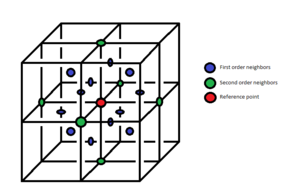These values agree with the numbers of first, second and third order neighbors a face centered cubic lattice is supposed to have, the result being clearly represented in fig. 9.

JC: Good idea to calculate the lattice parameter from each of the first three peaks and then compare with initial lattice constant, this confirms that the simulation is producing an fcc lattice. You needed to include plots of the RDF and integral of the RDF and then explain the differences between them - solid has long range order, liquid has short range order etc. There should be 24 third nearest neighbours, not 42 (42-12-6 = 24).

Dynamical properties and the difusion coefficient

Mean squared displacement

Figure 10: Mean squared deviation as a function of timestep for a solid

Figure 11: Mean squared deviation as a function of timestep for a liquid

Figure 12: Mean squared deviation as a function of timestep for a gas

Figure 13: Mean squared deviation as a function of timestep for a solid from a 1 milion atom simulation

Figure 14: Mean squared deviation as a function of timestep for a liquid from a 1 milion atom simulation

Figure 15: Mean squared deviation as a function of timestep for a gas from a 1 milion atom simulation

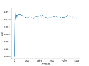
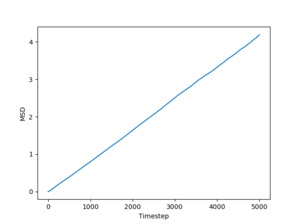
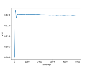
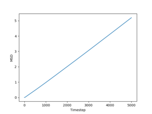
Figs. 10 to 15 show the evolution of the MSD with timestep for all three phases. The reason this quantity is so important is that it can be used to estimate the diffusion coefficient using the following equation:

$D=\frac{1}{6}\frac{d<r^2>}{dt}$

The simulated data will give a diffusion coefficient in reduced units (for length) squared per timestep. Even so, these simulations still have the power to predict the differences between diffusion through a solid, liquid and gas respectively.

Just by having a quick look at the graphs one can see that for solids and liquids the mean squared deviation stabilizes very quickly. This happens because the initial configurations of the particles are cubic lattices, and the solid has an equilibrium structure which is very close to this idealized structure, represented by the lattice. The liquid is not very far away from the lattice either, but for this phase the positions of the atoms inside the lattice are no longer well defined. In fact, this also leads to a deformation of the lattice, which is responsible for liquid flow. For a gas, on the other hand, the diffusion coefficient (proportional to the slope of the MSD) stabilizes more slowly, because the gas has a lower density than the liquid, so the particles in the system has to travel more (on average) in order to make the substance homogeneous. Finally, the average slopes for the three phases show that for solids the diffusion coefficient is effectively 0, which is correct, considering that nothing diffuses through a solid in a reasonable amount of time. For liquids and gases the simulation shows a constant diffusion coefficient, larger for gasses than for liquids. Again, this is perfectly reasonable. Estimates of the diffusion coefficients and their standard deviations from the plots shown above (for 1 milion atoms) are:

$$\begin{gathered} D_{solid}=-1.6550*10^{-8} \\ std=1.42*10^{-10} \\ (effectively \\ 0) \end{gathered}$$

$$\begin{gathered} D_{liquid}=1.7166*10^{-4} \\ std=2.78*10^{-8} \end{gathered}$$

$$\begin{gathered} D_{gas}=0.0060 \\ std=3.50*10^{-6} \end{gathered}$$

JC: Show the lines of best fit that you used to calculate D on the graphs, did you just fit to the linear part? The gas MSD takes longer before it becomes linear because collisions are more infrequent, not because particles begin on a lattice, initially the gas motion is ballistic, not diffusive.

Velocity autocorrelation function

The normalized velocity autocorrelation function is given by:

$C(\tau )=\frac{\underset{-\mathrm{\infty }}{\overset{\mathrm{\infty }}{\int }}v(t)v(t+\tau )dt}{\underset{-\mathrm{\infty }}{\overset{\mathrm{\infty }}{\int }}{v}^2(t)dt}$

For the 1D harmonic oscillator the velocity is given by the derivative of the position with respect to time, so it is:

$v(t)=-\omega A\sin (\omega t+\varphi )$

The autocorrelation function then becomes:

$C(\tau )=\frac{{\omega }^2{A}^2\underset{-\mathrm{\infty }}{\overset{\mathrm{\infty }}{\int }}\sin (\omega t+\varphi )\sin (\omega t+\varphi +\omega \tau )dt}{{\omega }^2{A}^2\underset{-\mathrm{\infty }}{\overset{\mathrm{\infty }}{\int }}{\sin }^2(\omega t+\varphi )dt}$

$C(\tau )=\frac{\underset{-\mathrm{\infty }}{\overset{\mathrm{\infty }}{\int }}\sin (\omega t+\varphi )\sin (\omega t+\varphi +\omega \tau )dt}{\underset{-\mathrm{\infty }}{\overset{\mathrm{\infty }}{\int }}{\sin }^2(\omega t+\varphi )dt}$

$C(\tau )=\frac{\underset{-\mathrm{\infty }}{\overset{\mathrm{\infty }}{\int }}\sin (\omega t+\varphi )[\sin (\omega t+\varphi )\cos (\omega \tau )+\sin (\omega \tau )\cos (\omega t+\varphi )]dt}{\underset{-\mathrm{\infty }}{\overset{\mathrm{\infty }}{\int }}{\sin }^2(\omega t+\varphi )dt}$

$C(\tau )=\frac{\cos (\omega \tau )\underset{-\mathrm{\infty }}{\overset{\mathrm{\infty }}{\int }}{\sin }^{}(\omega t+\varphi )dt+\sin (\omega \tau )\underset{-\mathrm{\infty }}{\overset{\mathrm{\infty }}{\int }}\sin (\omega t+\varphi )\cos (\omega t+\varphi )dt}{\underset{-\mathrm{\infty }}{\overset{\mathrm{\infty }}{\int }}{\sin }^2(\omega t+\varphi )dt}$

$C(\tau )=\frac{\cos (\omega \tau )\underset{-\mathrm{\infty }}{\overset{\mathrm{\infty }}{\int }}{\sin }^{}(\omega t+\varphi )dt+\frac{1}{2}\sin (\omega \tau )\underset{-\mathrm{\infty }}{\overset{\mathrm{\infty }}{\int }}\sin [2(\omega t+\varphi )dt]}{\underset{-\mathrm{\infty }}{\overset{\mathrm{\infty }}{\int }}{\sin }^2(\omega t+\varphi )dt}$

$C(\tau )=\frac{\cos (\omega \tau )\underset{-\mathrm{\infty }}{\overset{\mathrm{\infty }}{\int }}{\sin }^{}(\omega t+\varphi )dt}{\underset{-\mathrm{\infty }}{\overset{\mathrm{\infty }}{\int }}{\sin }^2(\omega t+\varphi )dt}+\frac{\sin (\omega \tau )\underset{-\mathrm{\infty }}{\overset{\mathrm{\infty }}{\int }}\sin [2(\omega t+\varphi )]dt}{\underset{-\mathrm{\infty }}{\overset{\mathrm{\infty }}{\int }}{\sin }^2(\omega t+\varphi )dt}$

Calculating the first integral:

$THeraputichorticulturelearningdifficulties\underset{-\mathrm{\infty }}{\overset{\mathrm{\infty }}{\int }}\sin [2(\omega t+\varphi )]dt=\frac{1}{2\omega }\underset{-\mathrm{\infty }}{\overset{\mathrm{\infty }}{\int }}\sin (x)dx=0$

The integral above is 0 because the integrand is an odd function and the integration interval is symmetric with respect to the origin. Therefore, only the first term remains, so the autocorrelation function becomes:

$C(\tau )=\underset{n\to \mathrm{\infty }}{\lim }\frac{\cos (\omega \tau )\underset{-n\pi }{\overset{n\pi }{\int }}{\sin }^{}(\omega t+\varphi )dt}{\underset{-n\pi }{\overset{n\pi }{\int }}{\sin }^2(\omega t+\varphi )dt}$

$C(\tau )=\cos (\omega \tau )$

JC: Correct.

Figure 16: Velocity autocorrelation function for the solid, liquid and harmonic oscillator

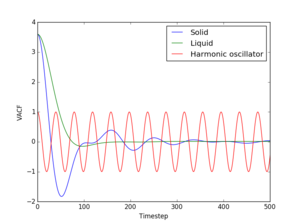The fact that the VACFs go to 0 for the solid and liquid phases is caused by collisions between the constituent particles. Upon many of these collisions velocities start taking random values and orientations, they are no longer correlated. However, atom vibrations in a solid are quite ordered, so the solid VACF does not approach 0 that quickly. For liquid, on the other hand, the motion is less ordered, so the VACF bacomes almost 0 immediately after the first peak occurs. From the harmonic motion it can be seen that the minima in the autocorrelation function occur at the moment when the spring attached to the oscillating is at maximum compression. Immediately after such a minimum the spring starts expanding. Consequently, the position of the first peak both in the solid and liquid VACF is an estimate of the time of the first collision. A 1D harmonic oscillator can vibrate at only one frequency at a time. This can also be seen from the Fourier transform of the autocorrelation function, which is known to be a delta function centered at that particular frequency. If the solid is approximated to a series of masses linked by springs (Einstein condensate) then it becomes obvious that it can have more than one vibrational frequency. In fact, this can be seen in the Fourier transform of the VACF, which gives an entire range of frequencies, and has an amplitude proportional to the number of states corresponding to each frequency. The Fourier transforms are shown in Fig. 17.

Figure 17: Fourier transforms of the VACFs of the solid and liquid phases

JC: Nice idea to calculate the Fourier transforms, but did you plot the running integral of the VACF or calculate the diffusion coefficients from the running integrals?

References

- ↑ Chueh, C. F., & Swanson, A. C. (1973, October). Estimation of liquid heat capacity. The Canadian Journal of Chemical Engineering. Wiley Subscription Services, Inc., A Wiley Company. https://doi.org/10.1002/cjce.5450510511