JC: General comments: Your python code was well written and commented, however, you missed quite a few marks by not finishing all of the tasks.

Programming for Simple Simulations

Introduction to the Ising Model

Task 1:

Consider a single lattice site within a 1-dimensional lattice: The lattice site has its own spin (si) and has two neighbors (sj), each with their own spins. Applying this within the equation for the interaction energy:

$- \frac{1}{2} J s_{i} \cdot 2 s_{j}$

In order to minimize the energy (achieve the most negative value) the spins si and sj must be parallel (both +1 or -1) thus giving:

$E = - J$

Hence for N lattice sites:

$E = - N J$

Applying this to higher dimensions:

2-D (4 sj neighbors): $E = - 2 N J$

3-D (6 sj neighbors): $E = - 3 N J$

Thus, considering the value of the energy in relation to the number of dimensions:

$E = - D N J$

Where D is the number of dimensions of the lattice.

For the multiplicity, 2 states (spin up/down) are available, but only one is occupied (si and sj parallel). Hence, using the statistical definition of multiplicity:

$W = \frac{N!}{N! 0!} = 1$

Thus making the entropy:

$S = k_{B} \ln W = 0$

JC: The multiplicity is 2 because there are 2 possible ground states, all spins pointing up or all spins pointing down. Therefore you should get W = 2 and S = 9.57e-24 J K-1.

Task 2:

Consider the flipped-spin lattice site, surrounded by its 6 neighbors, in 3-dimensions:

Where si is the flipped-spin lattice site, sj are its neighbors and so are the outer lattice points (not directly interacting with si).

The total energy of the lattice should therefore correspond to the sum of the interaction energies:

$E = E s_{i} + E s_{j} + E s_{o}$

Using our equation for the interaction energy between si, sj and so:

$- \frac{1}{2} J (6 s_{i} s_{j} + 6 s_{j} (5 s_{o} + s_{i}) + 993 s_{o} (s_{j} + 5 s_{o}))$

For the sake of calculation, it shall be assumed that si = -1 and sj and so = 1. Hence:

$- \frac{1}{2} J (- 6 + 24 + 5598)$

JC: I think the last term is this expression should be 5958 (= 993 x 6).

Assuming J=1.0

$E = - 2808$

JC: Nice method to work out the energy, your answer would have been correct if it wasn't for the typo in your expression above (writing 5598 instead of 5958).

Using the same principles as in Task 1 for the entropy (N = 1000):

$\frac{1000!}{999! 1!} = \frac{1000 \cdot 999 \cdot 998 . . .}{999 \cdot 998 . . .} = 1000$

JC: The multiplicity should be W = 2N; the flipped spin can be any one of the 1000 lattice sites and can either be pointing down with all other spins pointing up or vice versa.

Hence:

$S = k_{B} \ln W = 9.53 \cdot 1 0^{- 23}$

JC: This value is correct for the entropy gain because your error in calculating the multiplicity of the ground state and of the single spin flipped state cancel (missing factor of 2 in both cases).

Task 3:

Since magnetisation $= \sum s_{i}$

For the 1-D lattice: Magnetization $= + 3 - 2 = 1$

For the 2-D lattice: Magnetisation $= + 13 - 12 = 1$

At absolute zero, the entropy must be minimized. Hence, the lattice spins must be parallel. Thus the magnetization would be 1000.

JC: Correct, remember that the magnetisation can be positive or negative depending on whether the spins are pointing up or down, so M = +/- 1000 at absolute zero.

Calculating the Energy and Magnetization

Task 1:

energy() function

   def energy(self):
           total_int_e=0 # Empty variable for use in running sum
           for i,j in enumerate(self.lattice): # Enumeration used to develop i(row) and k(column) indexing.
               for k,l in enumerate(j):
                   u_neighbour=self.lattice[i-1,k] # Determining and accounting for neighbouring lattice sites
                   l_neighbour=self.lattice[i,k-1] # (l_neighbour: neighbour to the left of the lattice site under inspection).
                   if i==self.n_rows-1: # Accounting for the edge conditions (lattice is considered to be a repeating unit). 
                       d_neighbour=self.lattice[0,k]
                   if k==self.n_cols-1:
                       r_neighbour=self.lattice[i,0]
                   if k<self.n_cols-1:
                       r_neighbour=self.lattice[i,k+1]
                   if i<self.n_rows-1:
                       d_neighbour=self.lattice[i+1,k]
                   neighbours=u_neighbour+l_neighbour+d_neighbour+r_neighbour #Adding up neighbour interactions.  
                   total_int_e = total_int_e + self.lattice[i,k]*(neighbours) # Updating running sum of energy.
           energy=-0.5*1.0*total_int_e 
           return(energy)

magnetistion() function

   def magnetisation(self):
           magnetisation=0 # Empty variable for use in running sum.
           for layer in self.lattice: # Adding up each spin as the for loops iterate through the lattice.
               for spin in layer:
                   magnetisation=magnetisation+spin
           return(magnetisation)

JC: Good implementation of the periodic boundary conditions, code looks correct and is clearly commented.

Task 2:

ILcheck.py file output.

Consistent with the previous conclusions: Neighbour spins parallel at low energy states, opposed at high energy states. Regions of localized, parallel spins at intermediate energy states (analogous to ferromagnetic materials).

JC: Your energy/magnetisation functions are clearly working properly.

Introduction to the Monte Carlo Simulation

Task 1:

The number of configurations is given via the number of spins and the number of states available. Since there are only 2 spin states (up/down) and 100 spins:

$Number of configurations = W = n^{N} = 1.27 \cdot 1 0^{30}$

Dividing this by the number of configurations assessed per second gives the number of seconds required to assess all configurations:

$\frac{1.27 \cdot 1 0^{30}}{1 0^{9}} = 1.27 \cdot 1 0^{21} seconds$

JC: Values for number of configurations and time taken are correct, would be good to give the time taken in more intuitive units, e.g. years.

Task 2:

montecarlostep() Function

   def montecarlostep(self,T):
           E0 = self.energy() # Defining the un-flipped lattice energyagnetisation
           M0 = self.magnetisation()
           random_i = np.random.choice(range(0, self.n_rows)) # Choosing a random lattice site and flipping the spin. 
           random_j = np.random.choice(range(0, self.n_cols))
           select = self.lattice[random_i,random_j]
           flip = -1*select
           self.lattice[random_i,random_j]=flip
           E1 = self.energy() # Calculating the energy and magnetization of thelipped lattice. 
           M1 = self.magnetisation()
           d_E = E1 - E0 # Difference in energy
           if d_E < 0: # Condition: Energy difference is less than zero. Result: Keep new configuration
               self.E = self.E + E1
               self.M = self.M + M1
               self.E2 = self.E2 + E1**2
               self.M2 = self.M2 + M1**2
           if d_E > 0: 
               random_number = np.random.random()
               m_arg = -d_E/T
               if random_number <= np.exp(m_arg): # Condition: Randomly generated number is less or equal to the transition probabilty.
                   self.E = self.E + E1           # Result: Keep new configuration
                   self.M = self.M + M1
                   self.E2 = self.E2 + E1**2
                   self.M2 = self.M2 + M1**2
               if random_number > np.exp(m_arg):  # Condition: Randomly generated number is more than the transition probabilty.
                   self.E = self.E + E0           # Result: Reject new configuration
                   self.M = self.M + M0
                   self.E2 = self.E2 + E0**2
                   self.M2 = self.M2 + M0**2
                   self.lattice[random_i,random_j] *= -1 # Flipping the spin back to the previous lattice configuration
           self.n_cycles = self.n_cycles + 1 # Counting the number of Monte Carlo cycles as ILanim.py is run.
           return(self.energy(),self.magnetisation())

statistics() Function

   def statistics(self):
           a = self.E/self.n_cycles # Updating and reporting the parameters as they are processed via each Monte Carlo cycle.
           c = self.M/self.n_cycles
           b = self.E2/self.n_cycles
           d  = self.M2/self.n_cycles
           return(a,b,c,d, self.n_cycles)

JC: Monte Carlo and statistics code is correct.

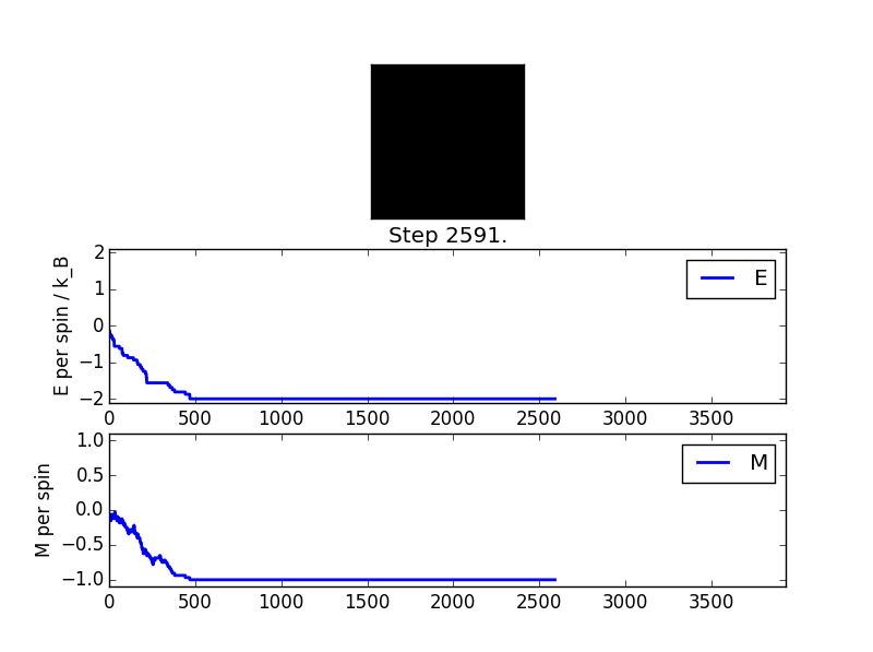
ILanim.py File Output

As it can be seen, the energy values plateau after 500 cycles. Comparing this with the 'black square' graphic (representing the lattice) indicates that the the simulation has reached an energy minimum (all spins parallel, energy does not decrease following repeated cycles).

statistics() function output

       Averaged quantities:
       E =  -1.83905527735
       E*E =  3.57797904228
       M =  -0.910294684129
       M*M =  0.887585468028
       n_cycles =  2596

Task 3:

Spontaneous magnetisation below the Curie Temperature (Tc) would not be expected as ferromagnetic materials below Tc have localised regions of aligned spins. Thus, lowering the energy and making their spins less likely to 'flip'. However, spontaneous magnetisation below Tc is a phenomenon that does occur due to spontaneous breaking of the global symmetry. At higher temperatures, the ferromagnet is stable at a symmetrical, potential energy minimum. This changes at lower temperatures (lower quantum energy levels) where even lower energy minima are available. However, accessing these energy levels requires a breaking of the lattice symmetry and thus a subsequent spin-flip and spontaneous magnetisation.

JC: Spontaneous magnetisation does occur below the Curie temperature as there is no longer enough thermal energy to disrupt the favourable parallel alignment of the spins.

Accelerating the Code

Task 1:

Runs: 36.253395524346274s, 37.24327775139553s, 36.18311255438408s, 36.95349178046948s, 35.97706749064636s

Average: 36.522069020248345s

Error: ±0.08073809958601577s

Task 2:

Modified energy() function

   def energy(self):
           rollup = np.roll(self.lattice, 1, 0) #Shifting the lattice indices upwards
           rollright = np.roll(self.lattice, 1, 1) #Shifting the lattice indices to the right 
           energyup = np.multiply(self.lattice,rollup) #Original lattice x rollup lattice gives the upper and lower neighbour interactions
           energyright = np.multiply(self.lattice,rollright) #As above, but for the left and right neighbours
           return(-sum(sum(energyup + energyright)))

The use of these roll functions (as opposed to for loops) simplify and shorten the code. Allowing faster calculations.

Modified magnetisation() function

   def magnetisation(self): #Simple use of the sum() function to add each spin element together.
           magnetisation = np.sum(self.lattice)
           return(magnetisation)

The same can be said for the sum function with regards to speeding up the simulation.

JC: Good use of numpy functions to speed up the code, you could also use the numpy sum function next to the "return" at the end of the energy code, rather than a double sum.

Task 3:

Runs: 2.08065802324227s, 2.044881977448931s, 2.0466643797304087s, 2.0339091634037274s, 2.096923004061445s

Average: 2.0606073095773563s

Error: ± 0.01670560549275668s

(Function runtime decreased by a factor of 17.7 seconds)

The Effect of Temperature

Task 1:

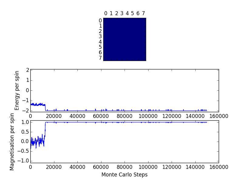
ILfinalframe_8x8_T=1.0 File Output

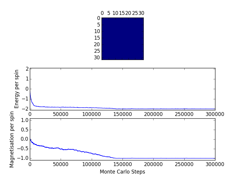
ILfinalframe_32x32_T=1.0 File Output

Comparing to the above 8x8 lattice, the number of cycles required to reach the equilibrium point increases with the size of the lattice. A larger lattice has a greater number of potential lattice spin flips. Thus, it would take much longer (more randomized cycles) to calculate the lowest energy state.

ILfinalframe.py_32x32_T=0.25 File Output

Decreasing the temperature appears to lower the number thermal fluctuations of the data (smoother curve) but has little effect on the required number of cycles below the Curie Temperature. (Above the Curie Temperature the lattice displays paramagnetic behaviour resulting in no distinct energy minima when using this model.

Modified montecarlostep()

   def montecarlostep(self,T):
           E0 = self.energy() # Defining the un-flipped lattice energyagnetisation
           M0 = self.magnetisation()
           random_i = np.random.choice(range(0, self.n_rows)) # Choosing a random lattice site and flipping the spin. 
           random_j = np.random.choice(range(0, self.n_cols))
           select = self.lattice[random_i,random_j]
           flip = -1*select
           self.lattice[random_i,random_j]=flip
           E1 = self.energy() # Calculating the energy and magnetization of thelipped lattice. 
           M1 = self.magnetisation()
           d_E = E1 - E0 # Difference in energy
           if d_E < 0: # Condition: Energy difference is less than zero. Result: Keep new configuration
               if self.n_cycles >= 150000: # "Ignore the first 150000 cycles" restraint condition
                   self.E = self.E + E1
                   self.M = self.M + M1
                   self.E2 = self.E2 + E1**2
                   self.M2 = self.M2 + M1**2
           if d_E > 0: 
               random_number = np.random.random()
               m_arg = -d_E/T
               if random_number <= np.exp(m_arg): # Condition: Randomly generated number is less or equal to the transition probabilty.
                   if self.n_cycles >= 150000:
                       self.E = self.E + E1           # Result: Keep new configuration
                       self.M = self.M + M1
                       self.E2 = self.E2 + E1**2
                       self.M2 = self.M2 + M1**2
               if random_number > np.exp(m_arg):  # Condition: Randomly generated number is more than the transition probabilty.
                   self.lattice[random_i,random_j] *= -1 # Flipping the spin back to the previous lattice configuration
                   if self.n_cycles >= 150000: 
                       self.E = self.E + E0           # Result: Reject new configuration
                       self.M = self.M + M0
                       self.E2 = self.E2 + E0**2
                       self.M2 = self.M2 + M0**2
           self.n_cycles = self.n_cycles + 1 # Counting the number of Monte Carlo cycles as ILanim.py is run.
           return(self.energy(),self.magnetisation())

Modified statistics()

   def statistics(self):
           a = self.E/(self.n_cycles - 150000) # Updating and reporting the parameters as they are processed via each Monte Carlo cycle.
           c = self.M/(self.n_cycles - 150000) # Minus the 150000 cycles that are not at equilibrium.
           b = self.E2/(self.n_cycles - 150000)
           d = self.M2/(self.n_cycles - 150000)
           return(a,b,c,d,self.n_cycles)

JC: Cutoff implemented in code, however, the line "if self.n_cycles >= 150000:" should be changed to ">" not ">=" - what would happen if you ran a simulation of 150001 cycles with your current code? This error will be very small though as the number of values in your average increases.

Task 2:

Modified IL temperature code

   from IsingLattice import *
   from matplotlib import pylab as pl
   import numpy as np

   n_rows = 8 #Generating a randomised Ising Lattice as before 
   n_cols = 8
   il = IsingLattice(n_rows, n_cols)
   il.lattice = np.ones((n_rows, n_cols))
   spins = n_rows*n_cols
   runtime = 151000 # Setting the number of cycles = 1000 + the 150000 cycle restraint condition.
   times = range(runtime)
   temps = np.arange(0.25, 5, 0.25)
   energies = [] #Creating empty lists with which to store the output.
   magnetisations = []
   energysq = []
   magnetisationsq = []
   for t in temps:
       for i in times:
           energy, magnetisation = il.montecarlostep(t) #setting the required number of Monte Carlo iterations
       aveE, aveE2, aveM, aveM2, n_cycles = il.statistics() #reading and storing the output of the statistics function
       energies.append(aveE) 
       energysq.append(aveE2)
       magnetisations.append(aveM)
       magnetisationsq.append(aveM2)
       #reset the IL object for the next cycle
       il.E = 0.0
       il.E2 = 0.0
       il.M = 0.0
       il.M2 = 0.0
       il.n_cycles = 0
   E_error = (np.sqrt((np.array(energysq)-np.array(energies)**2))/(np.sqrt(n_cycles))/spins) #standard error calculations
   M_error = (np.sqrt((np.array(magnetisationsq)-np.array(magnetisations)**2))/(np.sqrt(n_cycles))/spins)
   fig = pl.figure() #Graph plots + Error bars
   enerax = fig.add_subplot(2,1,1)
   enerax.set_ylabel("Energy per spin")
   enerax.set_xlabel("Temperature")
   enerax.set_ylim([-2.1, 2.1])  
   magax = fig.add_subplot(2,1,2)
   magax.set_ylabel("Magnetisation per spin")
   magax.set_xlabel("Temperature")
   magax.set_ylim([-1.1, 1.1])
   enerax.errorbar(temps, np.array(energies)/spins,yerr=E_error)
   magax.errorbar(temps, np.array(magnetisations)/spins,yerr=M_error)
   pl.show()

   final_data = np.column_stack((temps, energies, energysq, magnetisations, magnetisationsq))
   np.savetxt("8x8.dat", final_data) #saving the output

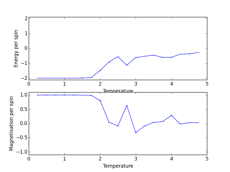
ILtemperature file output

The energy per spin seems to increase, non-uniformly, with temperature. In the context of ferromagnets, as the Curie temperature is approached, a smaller number of the lattice spins are parallel, causing their interaction energies to increase. The increased temperature raises the thermal energy of each spin which reduces the strength of the interaction between neighbouring spins, leading to a loss of stabilization energy.

JC: How many Monte Carlo steps did you use and why?

The Effect of System Size

Task:

Effect of system size on energy:

   def systemsizeE(): 
       from matplotlib import pylab as pl
       import numpy as np

       spins_2 = 2*2 #defining the number of spins in each lattice
       spins_4 = 4*4
       spins_8 = 8*8
       spins_16 = 16*16
       spins_32 = 32*32

       a = np.loadtxt('2x2.dat') #Reading each lattice file
       b = np.loadtxt('4x4.dat')
       c = np.loadtxt('8x8.dat')
       d = np.loadtxt('16x16.dat')
       e = np.loadtxt('32x32.dat')

       temps = [] #defining an array of temperature data
       for i in a:
           temps.append(i[0])
       T = np.array(temps)

       energies_2x2 = [] #defining arrays for the energy data of each lattice using the loadtxt() output.
       for i in a:
           energies_2x2.append(i[1])
       E_2 = np.array(energies_2x2)

       energies_4x4 = []
       for i in b:
           energies_4x4.append(i[1])
       E_4 = np.array(energies_4x4)

       energies_8x8 = []
       for i in c:
           energies_8x8.append(i[1])
       E_8 = np.array(energies_8x8)

       energies_16x16 = []
       for i in d:
           energies_16x16.append(i[1])
       E_16 = np.array(energies_16x16)

       energies_32x32 = []
       for i in e:
            energies_32x32.append(i[1])
       E_32 = np.array(energies_32x32)

       pl.ylabel("Energy per spin") #plotting the energy (per spin) against the temperature values
       pl.xlabel("Temperature")
       pl.plot(T,E_2/spins_2,'r',T,E_4/spins_4,'g',T,E_8/spins_8,'b',T,E_16/spins_16,'y',T,E_32/spins_32,'c')
       pl.show()

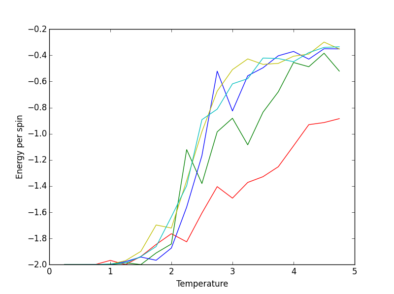
ILtemperature file output: red=2x2, green=4x4, blue=8x8, yellow=16x16, cyan=32x32.

JC: Loadtxt function used correctly.

^{All of the plots start at the same point on the plots. This is due to them all being at their respective equilibrium configurations (using the 150000 cycle deduction) and thus have their energies minimised to the same degree. The larger lattices ascend to higher energies, with temperature, much faster than their smaller counterparts. This is most likely due to the larger lattices having a greater number of possible 'flipped-spin' configurations which means that for a set temperature, there is potential for a greater number of non-parallel spins in a larger lattice compared to a smaller lattice. Thus, raising the energy per spin. However, an upper energy limit can be observed for the lattices (8x8, 16x16, 32x32 have similar distributions at higher temperatures). This may indicate a common state that all of the lattices occupy at this temperature which possibly may indicate a crossing of the Curie Temperature (phase transition), where the material becomes paramagnetic and receives no stabilisation via spin-spin interactions. In such a situation, the lattice size would be irrelevant and may explain why the larger lattices converge towards the same energy. However, this does not explain why the smaller lattices (2x2 and 4x4) do not converge to the same point.}

JC: Well noticed that lattice sizes of 8x8 and above converge.

Effect of system size on magnetisation:

   def systemsizeM(): # As above, but using the magnetisation values of the loadtxt output.
       from matplotlib import pylab as pl
       import numpy as np

       spins_2 = 2*2
       spins_4 = 4*4
       spins_8 = 8*8
       spins_16 = 16*16
       spins_32 = 32*32

       a = np.loadtxt('2x2.dat')
       b = np.loadtxt('4x4.dat')
       c = np.loadtxt('8x8.dat')
       d = np.loadtxt('16x16.dat')
       e = np.loadtxt('32x32.dat')

       temps = []
       for i in a:
           temps.append(i[0])
       T = np.array(temps)

       mags_2x2 = []
       for i in a:
           mags_2x2.append(i[3])
       M_2 = np.array(mags_2x2)

       mags_4x4 = []
       for i in b:
           mags_4x4.append(i[3])
       M_4 = np.array(mags_4x4)

       mags_8x8 = []
       for i in c:
           mags_8x8.append(i[3])
       M_8 = np.array(mags_8x8)

       mags_16x16 = []
       for i in d:
           mags_16x16.append(i[3])
       M_16 = np.array(mags_16x16)

       mags_32x32 = []
       for i in e:
           mags_32x32.append(i[3])
       M_32 = np.array(mags_32x32)

       pl.ylabel("Energy per spin")
       pl.xlabel("Temperature")
       pl.plot(T,M_2/spins_2,'r',T,M_4/spins_4,'g',T,M_8/spins_8,'b',T,M_16/spins_16,'y',T,M_32/spins_32,'c')
       pl.show()

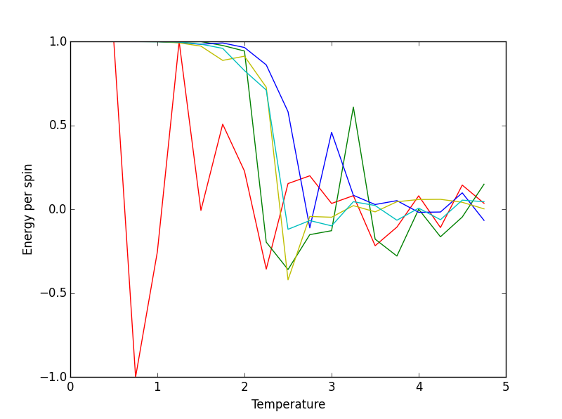
SystemsizeM File Output: red=2x2, green=4x4, blue=8x8, yellow=16x16, cyan=32x32.

JC: Be careful with axis labels, is this magnetisation?

The magnetisation (aside from some large fluctuations in the 2x2 plot) decreases from a maximum value of which all of the the lattice sizes share. This refers to the equilibrium state where all of the lattice spins are parallel, leading to the maximum degree of magnetisation. As the temperature is increased however, the thermal energy of each spin is raised, the spin-spin stabilisation interactions become weaker, and the material starts to become paramagnetic which results in a loss of magnetisation. This is represented in the systemsizeM plot as we see each of the plots converge to a magnetisation value of 0 (per spin) as the temperature is increased.

JC: How does the temperature of the phase transition change with system size?

Calculating the Heat Capacity

Task 1:

$C_{v} = (\frac{\partial E}{\partial T})$

Considering E (internal energy) with respect to the temperature (constant volume):

$C_{v} = \frac{\partial}{\partial T} (\frac{\sum E e x p (- E / k_{B} T))}{\sum e x p (- E / k_{B} T)})$

Using the quotient rule of differentiation:

$a = \sum E e x p (- E / k_{B} T)$

$b = \sum e x p (- E / k_{B} T)$

$C_{v} = \frac{b \frac{d a}{d T} - a \frac{d b}{d T}}{b^{2}}$

Calculating and simplifying:

$C_{v} = \frac{1}{k_{B} T^{2}} (\frac{\sum E^{2} e x p (- E / k_{B} T))}{\sum e x p (- E / k_{B} T)} - (\frac{\sum E e x p (- E / k_{B} T))}{\sum e x p (- E / k_{B} T)})^{2})$

Note that:

$< E^{2} > = \frac{\sum E^{2} e x p (- E / k_{B} T))}{\sum e x p (- E / k_{B} T)}$

$< E > = \frac{\sum E e x p (- U / k_{B} T))}{\sum e x p (- E / k_{B} T)}$

Since Variance is defined as $< E^{2} > - < E >^{2}$

$C_{v} = \frac{V a r [E]}{k_{B} T}$

JC: Good, clear derivation.

Task 2:

def heatcapacity(): #As with the previous systemsize() functions, but using the outputs to calculate the heat capacity.

JC: Show the actual code that you used.

   from matplotlib import pylab as pl
   import numpy as np

   a = np.loadtxt('2x2.dat')
   b = np.loadtxt('4x4.dat')
   c = np.loadtxt('8x8.dat')
   d = np.loadtxt('16x16.dat')
   e = np.loadtxt('32x32.dat')

   temps = []
   for i in a:
       temps.append(i[0])
   T = np.array(temps)

   energies_2x2 = []
   for i in a:
       energies_2x2.append(i[1])
   E_2 = np.array(energies_2x2)

   energysq_2x2 = []
   for i in a:
       energysq_2x2.append(i[2])
   Es_2 = np.array(energysq_2x2)

   Cv_2 = (Es_2 - (E_2**2))/(T**2) #heat capacity calculation for the 2x2 lattice (And so on for each lattice size). Note that we are working in reduced units. Hence there is no need to consider the boltzmann constant.

   energies_4x4 = []
   for i in b:
       energies_4x4.append(i[1])
   E_4 = np.array(energies_4x4)

   energysq_4x4 = []
   for i in b:
       energysq_4x4.append(i[2])
   Es_4 = np.array(energysq_4x4)

   Cv_4 = (Es_4 - (E_4**2))/(T**2)

   energies_8x8 = []
   for i in c:
       energies_8x8.append(i[1])
   E_8 = np.array(energies_8x8)

   energysq_8x8 = []
   for i in c:
       energysq_8x8.append(i[2])
   Es_8 = np.array(energysq_8x8)

   Cv_8 = (Es_8 - (E_8**2))/(T**2)

   energies_16x16 = []
   for i in d:
       energies_16x16.append(i[1])
   E_16 = np.array(energies_16x16)

   energysq_16x16 = []
   for i in d:
       energysq_16x16.append(i[2])
   Es_16 = np.array(energysq_16x16)

   Cv_16 = (Es_16 - (E_16**2))/(T**2)

   energies_32x32 = []
   for i in e:
       energies_32x32.append(i[1])
   E_32 = np.array(energies_32x32)

   energysq_32x32 = []
   for i in e:
       energysq_32x32.append(i[2])
   Es_32 = np.array(energysq_32x32)

   Cv_32 = (Es_32 - (E_32**2))/(T**2)

   pl.ylabel("Heat Capacity") 
   pl.xlabel("Temperature")
   pl.plot(T,Cv_2,'r') #plotting separate graphs due to the large differences in y axis maxima (2x2 graph is heavily skewed otherwise)
   pl.show()
   pl.ylabel("Heat Capacity") 
   pl.xlabel("Temperature")
   pl.plot(T,Cv_4,'g')
   pl.show()
   pl.ylabel("Heat Capacity") 
   pl.xlabel("Temperature")
   pl.plot(T,Cv_8,'b')
   pl.show()
   pl.ylabel("Heat Capacity") 
   pl.xlabel("Temperature")
   pl.plot(T,Cv_16,'y')
   pl.show()
   pl.ylabel("Heat Capacity") 
   pl.xlabel("Temperature")
   pl.plot(T,Cv_32,'c')
   pl.show()

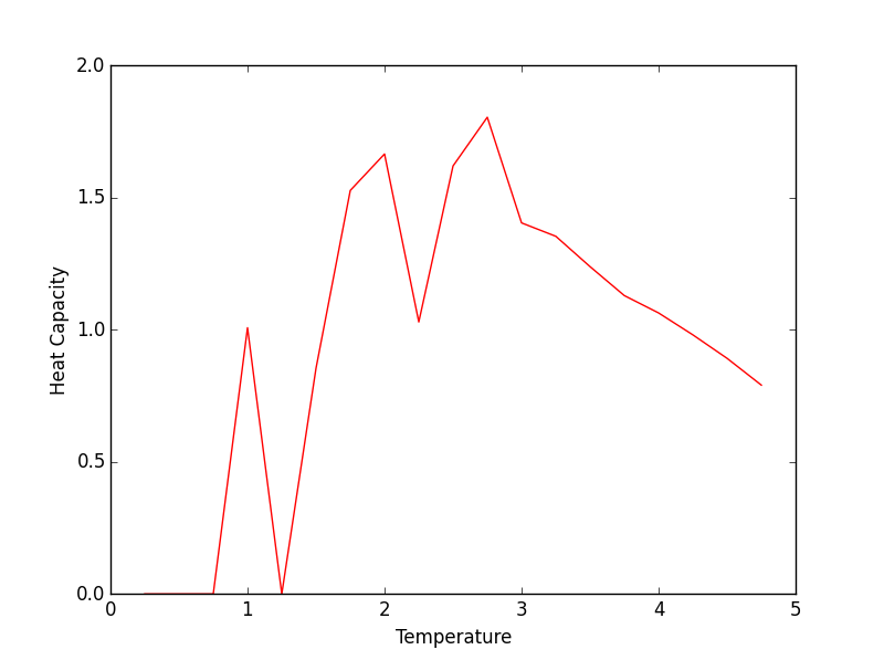
2x2 Heat Capacity plot

4x4 Heat Capacity plot

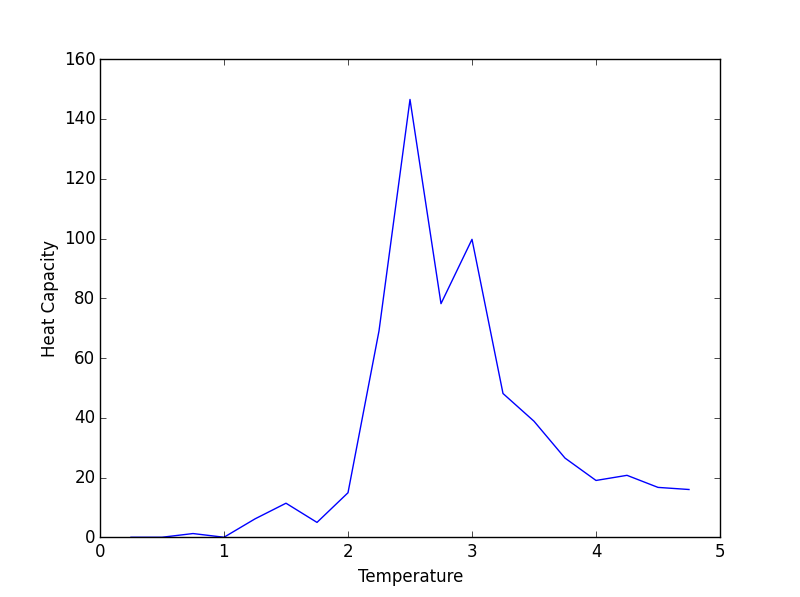
8x8 Heat Capacity plot

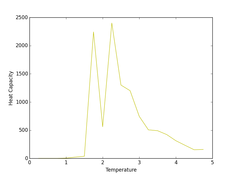
16x16 Heat Capacity plot

32x32 Heat Capacity plot

Aside from some thermal fluctuations, the all of the heat capacities share a common maximum between temperatures of 2 and 3 (working in reduced units). The height of this maximum increases with increasing lattice size which coincides with the concept of heat capacity being an extensive property. Thus, a larger lattice can absorb more thermal energy than a smaller one. This may explain why the smaller lattices reached lower maximum energies (in the systemsizeE plot) than their larger counterparts for a given temperature range.

JC: Plot the heat capacities for the different system sizes on the same axes so that it is easier to compare them.

Talk:Mod:Liam python Y3

Programming for Simple Simulations

Introduction to the Ising Model

Task 1:

Task 2:

Task 3:

Calculating the Energy and Magnetization

Task 1:

Task 2:

Introduction to the Monte Carlo Simulation

Task 1:

Task 2:

Task 3:

Accelerating the Code

Task 1:

Task 2:

Task 3:

The Effect of Temperature

Task 1:

Task 2:

The Effect of System Size

Task:

Calculating the Heat Capacity

Task 1:

Task 2:

Locating the Curie Temperature

Task 1:

Task 2:

Task 3:

Task 4: