Talk:Mod:KS5214LS

JC: General comments: Simulation results look good and all task answered. Try to make your answers more concise and focus on answering the question, referring specifically to your own results, rather than making general comments.

Introduction to Molecular Dynamics Simulation

Molecular Dynamics Simulations aim to describe how a set of atoms move over time, using classical mechanics. Whilst the simulation carried out here are of simple systems, MDS can be used to further understand complex systems such as biological systems. Here the Large-scale Atomic/Molecular Massively Parallel Simulator (LAMMPS) was used in order to simulate the movement of the particles with respect to time using the velocity-Verlet algorithm. This allowed us to model the movement of atoms and extract thermodynamic properties. It also clearly portrayed the limitations of the program and the approximations used, especially when it comes to vapor and solid systems as it was proven that the approximations used provide reasonable and comparable results for liquid systems, but large discrepancies for vapor and solid phases.

Numerical Integration

TASK: Open the file HO.xls. In it, the velocity-Verlet algorithm is used to model the behaviour of a classical harmonic oscillator. Complete the three columns "ANALYTICAL", "ERROR", and "ENERGY".

The position of the classical harmonic oscillator as a function of time was determined using:

$x\left(t\right)=A\cos (\omega t+\varphi )$

with $A=1.0$, $\omega =1.0$, and $\varphi =0.0$ yielding an analytical solution to the position, which as seen from Figure 1 below, seems to be in agreement with the Velocity-Verlet algorithm.

Figure 1:Position of a classical harmonic oscillator as a function of time (timestep=0.1)

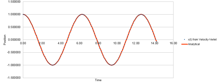
It is worth noting that the velocity and acceleration of a simple harmonic oscillator oscillate with the same frequency as the position, but with shifted phases. In simple harmonic motion when the displacement is maximum the velocity is at zero and when the displacement is zero, the velocity is at maximum. The acceleration on the other hand is at maximum when the displacement is at maximum and it is at zero when displacement is at 0.

The energy of the classical harmonic oscillator was then determined using:

$E=\frac{1}{2}m{v}^2+\frac{1}{2}k{x}^2$

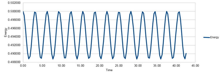
with $m=1.0$, $k=1.0$ and $x\left(t\right)$ affording Figure 2.

Figure 2:Energy of a classical harmonic oscillator as a function of time (timestep=0.1)

The result obtained (Figure 2) is a periodic motion, repeated in a sinusoidal fashion. It maintains a constant amplitude, with a range between 0.5000 and 0.499. The harmonic oscillator has a period of 6.50 (time of single oscillation) and a frequency of 0.154 (number of cycles per unit time). The position at a given time, t depends on the phase, φ, which was predetermined to 0.00, giving the starting point on the sine wave, the period and frequency are determined by the size of the mass, m (m=1.00) and the force constant, k (k=1.00) whilst the amplitude and phase are determined by the starting position, X(0) (X(0)=1.00) and velocity, V(0) (V(0)=0.00). For an ideal harmonic oscillator, the total energy would be expected to be constant therefore the simulation does not provide an ideal result. However the fluctuation is of a magnitude of 0.00149 energy units, which approximates to 0.25% of the energy therefore the error is small and the physical behavior predicted can be considered acceptable for the purposes of the experiment.

TASK: For the default timestep value, 0.1, estimate the positions of the maxima in the ERROR column as a function of time. Make a plot showing these values as a function of time, and fit an appropriate function to the data.

Figure 3 shows the discrepancy between the classical, analytical solution and the solution from the Velocity-Verlet algorithm. Whilst Figure 1 shows an agreement between the Valocity-Verlet algorithm and the analytical calculation, Figure 3 suggest that there is a small variation between the two solutions and thus the Velocity-Verlet algorithm results to an error in the caclulation. The error is biggest for values of time that give position close to 0, and error at these points increases linearly with time according to:

$(y=4.18*10^{-4}\cdot t+3.81*10^{-5})$

This linear increase in error is due to the Taylor expansion of the integral used in the Velocity-Verlet algorith.

JC: The increase in the error is due to accumulation of error over time. Why does the error oscillate?

Figure 3: Linear fit to Error Function Maxima

TASK: Experiment with different values of the timestep. What sort of a timestep do you need to use to ensure that the total energy does not change by more than 1% over the course of your "simulation"? Why do you think it is important to monitor the total energy of a physical system when modelling its behaviour numerically?

It was found that the sinusoidal fluctuation of the energy increases with increasing timesteps. On the other hand, the absolute value of the energy decreases. As aforementioned for a timestep of 0.10, the fluctuation is very small of 0.25% energy change. As the timestep increases to 0.20 and 0.30 the fluctutaions produced are 1.00% and 2.00% of energy respectively. The 0.20 timestep was found to be the limiting value with fluctuations at 1.00% (figure XX) and therefore, a timestep below 0.20 has to be chosen in order to keep energy fluctuations less that 1.00%.

It is important to monitor the total energy when performing the simulations as energy is meant to be constant over time.

Figure 4:Energy of a classical harmonic oscillator as a function of time (timestep=0.2)

Figure 5:Energy of a classical harmonic oscillator as a function of time (timestep=0.3)

It is important to monitor the total energy of a physical system when modelling its behaviour numerically because only when the system obeys physical laws (energy conservation in this case) to a certain extent, the outputs of the simulation can be considered meaningful.

JC: Good choice of timestep and explanation.

Atomic Forces

TASK: For a single Lennard-Jones interaction, $\varphi \left(r\right)=4ϵ(\frac{{\sigma }^{12}}{r^{12}}-\frac{{\sigma }^6}{r^6})$, find the separation, $r_0$, at which the potential energy is zero.

$\varphi \left(r_0\right)=0$

$4ϵ(\frac{{\sigma }^{12}}{r_0^{12}}-\frac{{\sigma }^6}{r_0^6})=0$

$\frac{{\sigma }^{12}}{r_0^{12}}-\frac{{\sigma }^6}{r_0^6}=0$

$\frac{{\sigma }^{12}}{r_0^{12}}=\frac{{\sigma }^6}{r_0^6}$

$\frac{{\sigma }^{12}}{{\sigma }^6}=\frac{r_0^{12}}{r_0^6}$

$r_0=\sigma$

The potential energy is 0 at $r_0=\sigma$.

What is the force at this separation?

For a single particle with $r=r_0=\sigma$:

$$\begin{gathered} F=-\frac{\text{d} \\ U\left(r^N\right)}{\text{d} \\ r} \end{gathered}$$

$$\begin{gathered} =-\frac{\text{d} \\ \varphi \left(r_0\right)}{\text{d} \\ {r}_0} \end{gathered}$$

$$\begin{gathered} =-\frac{d\left[4ϵ(\frac{{\sigma }^{12}}{r_0^{12}}-\frac{{\sigma }^6}{r_0^6})\right]}{\text{d} \\ {r}_0} \end{gathered}$$

$=-24ϵ(\frac{{\sigma }^6}{r_0^7}-\frac{2\cdot {\sigma }^{12}}{r_0^{13}})$

$=-24ϵ(\frac{r_0^6}{r_0^7}-\frac{2\cdot r_0^{12}}{r_0^{13}})$

$=\frac{48ϵ}{r_0}-\frac{24ϵ}{r_0}$

$=\frac{24ϵ}{r_0}$

At $r=r_0=\sigma$, the force is $F=\frac{24ϵ}{r_0}$.

Find the equilibrium separation, $r_{eq}$, and work out the well depth ($\varphi \left(r_{eq}\right)$).

The system is at equilibrium when F=0:

$F\left(r_{eq}\right)=0$

$$\begin{gathered} -\frac{\text{d} \\ \varphi \left(r_{eq}\right)}{\text{d} \\ {r}_{eq}}=0 \end{gathered}$$

$$\begin{gathered} -\frac{\text{d}\left[4ϵ(\frac{{\sigma }^{12}}{r_{eq}^{12}}-\frac{{\sigma }^6}{r_{eq}^6})\right]}{\text{d} \\ {r}_{eq}}=0 \end{gathered}$$

$-24ϵ(\frac{{\sigma }^6}{r_{eq}^7}-\frac{2\cdot {\sigma }^{12}}{r_{eq}^{13}})=0$

$\frac{{\sigma }^6}{r_{eq}^7}=2\cdot \frac{{\sigma }^{12}}{r_{eq}^{13}}$

$2{\sigma }^6=r_{eq}^6$

$$\begin{gathered} r_{eq}=\sqrt[6]{2} \\ \sigma \end{gathered}$$

Equilibrium separation is $$\begin{gathered} r_{eq}=\sqrt[6]{2} \\ \sigma \end{gathered}$$.

Using

$$\begin{gathered} r_{eq}=\sqrt[6]{2} \\ \sigma \end{gathered}$$

:

$$\begin{gathered} \varphi \left(r_{eq}\right)=4ϵ(\frac{{\sigma }^{12}}{{\left(\sqrt[6]{2} \\ \sigma \right)}^{12}}-\frac{{\sigma }^6}{{\left(\sqrt[6]{2} \\ \sigma \right)}^6})=4ϵ(\frac{1}{2^2}-\frac{1}{2})=-ϵ \end{gathered}$$

The well depth at $$\begin{gathered} r_{eq}=\sqrt[6]{2} \\ \sigma \end{gathered}$$ is $\varphi \left(r_{eq}\right)=-ϵ$.

Evaluate the integrals $\underset{2\sigma }{\overset{\mathrm{\infty }}{\int }}\varphi \left(r\right)\mathrm{d}r$, $\underset{2.5\sigma }{\overset{\mathrm{\infty }}{\int }}\varphi \left(r\right)\mathrm{d}r$, and $\underset{3\sigma }{\overset{\mathrm{\infty }}{\int }}\varphi \left(r\right)\mathrm{d}r$ when $\sigma =ϵ=1.0$.

For

$\sigma =ϵ=1.0$

:

$\underset{2\sigma }{\overset{\mathrm{\infty }}{\int }}\varphi \left(r\right)\text{d}r=\underset{2\sigma }{\overset{\mathrm{\infty }}{\int }}4ϵ(\frac{{\sigma }^{12}}{r^{12}}-\frac{{\sigma }^6}{r^6})\text{d}r=\underset{2}{\overset{\mathrm{\infty }}{\int }}4(\frac{1^{12}}{r^{12}}-\frac{1^6}{r^6})\text{d}r=4{(\frac{1}{5r^5}-\frac{1}{11r^{11}})}_2^{\mathrm{\infty }}=-2.48\cdot 10^{-2}$

$\underset{2.5\sigma }{\overset{\mathrm{\infty }}{\int }}\varphi \left(r\right)\text{d}r=4{(\frac{1}{5r^5}-\frac{1}{11r^{11}})}_{2.5}^{\mathrm{\infty }}=-8.18\cdot 10^{-3}$

$\underset{3\sigma }{\overset{\mathrm{\infty }}{\int }}\varphi \left(r\right)\text{d}r=4{(\frac{1}{5r^5}-\frac{1}{11r^{11}})}_3^{\mathrm{\infty }}=-3.29\cdot 10^{-3}$

JC: All maths correct and nicely laid out.

Periodic Boundary Conditions

TASK: Estimate the number of water molecules in 1mL of water under standard conditions. Estimate the volume of $10000$ water molecules under standard conditions.

At standard conditions $$\begin{gathered} \rho =999.7 \\ \frac{kg}{m^3}=0.9997 \\ \frac{g}{mL} \end{gathered}$$. Using Avogadro's number, $N_A=6.022\cdot 10^{23}mo{l}^{-1}$ and molar mass of water, $$\begin{gathered} M_{H_{2}O}=18 \\ g{mol}^{-1} \end{gathered}$$.

$$\begin{gathered} m=\frac{\rho }{V}=\frac{0.9997}{1}=0.9997 \\ g \end{gathered}$$

$$\begin{gathered} n=\frac{m}{M}=\frac{0.9997}{18}=0.055539 \\ mol \end{gathered}$$

$N=n\cdot N_A=0.055539\cdot 6.022\cdot 10^{23}=3.344\cdot 10^{22}$

At standard conditions there are approximately $3.344\cdot 10^{22}$ molecules in 1 mL water.

$$\begin{gathered} n=\frac{N}{N_A}=\frac{10,000}{6.022\cdot 10^{23}}=1.6606\cdot 10^{-20} \\ mol \end{gathered}$$

$$\begin{gathered} m=M\cdot n=18\cdot 1.6606\cdot 10^{-20}=2.9890\cdot 10^{-19} \\ g \end{gathered}$$

$$\begin{gathered} V=\frac{m}{\rho }=\frac{2.9890\cdot 10^{-19} \\ }{0.9997 \\ }=2.9899\cdot 10^{-19} \\ mL \end{gathered}$$

At standard conditions, 10,000 water molecules take up a volume of $$\begin{gathered} 2.9899\cdot 10^{-19} \\ mL \end{gathered}$$.

TASK: Consider an atom at position $(0.5,0.5,0.5)$ in a cubic simulation box which runs from $(0,0,0)$ to $(1,1,1)$. In a single timestep, it moves along the vector $(0.7,0.6,0.2)$. At what point does it end up, after the periodic boundary conditions have been applied?.

Without periodic boundary conditions, the atom would be outside the box after one timestep at position $(1.2,1.1,0.7)$. Applying periodic boundary conditions, results in the atom being at position $(0.2,0.1,0.7)$ inside the box.

Reduced Units

TASK: The Lennard-Jones parameters for argon are $$\begin{gathered} \sigma =0.34\mathrm{n}\mathrm{m},ϵ \\ / \\ {k}_B=120\mathrm{K} \end{gathered}$$. If the LJ cutoff is $r^{*}=3.2$, what is it in real units? What is the well depth in $$\begin{gathered} {\mathrm{k}\mathrm{J} \\ \mathrm{m}\mathrm{o}\mathrm{l}}^{-1} \end{gathered}$$? What is the reduced temperature $T^{*}=1.5$ in real units?

$r=r^{*}\cdot \sigma$

$$\begin{gathered} r=3.20\cdot 0.34 \\ =1.09 \\ nm \end{gathered}$$

$$\begin{gathered} {ϵ}_m=ϵ\cdot N_A=120 \\ {k}_B\cdot N_A \end{gathered}$$

$$\begin{gathered} {ϵ}_m=120 \\ \text{K}\cdot 1.381\cdot 10^{-26}\cdot 6.022\cdot 10^{23}=0.997 \\ kJ{mol}^{-1} \end{gathered}$$

$$\begin{gathered} T=\frac{T^{*}\cdot ϵ}{k_B}=1.50\cdot 120 \\ =180\text{K} \end{gathered}$$

JC: Good, all calculations correct and working clearly shown.

Equilibration

TASK: Why do you think giving atoms random starting coordinates causes problems in simulations? Hint: what happens if two atoms happen to be generated close together?

The number of atoms included in the box for the simulation is large. Giving atoms random starting coordinates results in a high probability of atoms placed in separation distances smaller than their equilibrium distance. This would result to very high interaction of atom pairs, with inaccurate and extremely high Lennard-Jones potential. As a result, the simulation would not be a good representation of the system, affording inaccurate results when measuring properties.

JC: High repulsive forces can make the simulation unstable and cause it to crash unless a much smaller timestep is used.

TASK: Satisfy yourself that this lattice spacing $(1.07722)$ corresponds to a number density of lattice points of $0.8$. Consider instead a face-centred cubic lattice with a lattice point number density of 1.2. What is the side length of the cubic unit cell?

Figure 6: Simple Cubic Lattice

Figure 7: Face Centered Cubic Lattice

Number density,ρ is defined as:

$\rho =\frac{n}{V}$

Volume, V can be calculated from the lattice spacing according to:

$x$: $V=x^3$.

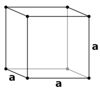
There is 1 lattice point per unit cell as seen from Figure 6 since $(8\cdot \frac{1}{8}=1)$.
The number density in a simple cubic lattice with side length x=1.07722 is therefore:

$\rho =\frac{n}{x^3}=\frac{1}{1.07722^3}=\frac{1}{1.25}=0.8$

In a fcc lattice (Figure 7) there are 4 lattice points per unit cell $(6\cdot \frac{1}{2}+8\cdot \frac{1}{8}=4)$.
This can be re-written as:

$x=\sqrt[3]{\frac{n}{\rho }}$

Using ρ=1.2 affords:

$x=\sqrt[3]{\frac{4}{1.2}}=1.49$

JC: Good.

TASK: Consider again the face-centred cubic lattice from the previous task. How many atoms would be created by the create_atoms command if you had defined that lattice instead?

As aforementioned there are four lattice points per unit cell in the face-centered cubic lattice, therefore the command:

region box block 0 10 0 10 0 10
create_box 1 box
create_atoms 1 box

would give four times the number of atoms, therefore: $4\cdot 10\cdot 10\cdot 10=4000$ atoms

Setting the Properties of the Atoms

TASK: Using the LAMMPS manual, find the purpose of the following commands in the input script:

mass 1 1.0
pair_style lj/cut 3.0
pair_coeff * * 1.0 1.0

mass 1 1.0 Sets the mass of all atoms of type '1' to 1.0.
pair_style lj/cut 3.0 Defines the interaction between atom pairs (pairwise interaction). In this case specifically, a Lennard-Jones potential will be used for a specific distance of 3.0 reduced units. The cut-off point is an approximation made when running the simulation, however 3.0 reduced units is considered a good approximation because the Lennard-Jones potential decreases rapidly with increasing distance. If no cut-off distance was defined, an infinite number of atomic interactions would need to be taken into account and computed in the periodic boundary conditions used in this investigation.
pair_coeff * * 1.0 1.0 defines the pairwise force field coefficients for all types of atoms (Note the use of asterisk (*) instead of specifying atom type(s). This is a wildcard including all atom types) in the simulation. In this case the coefficients are all 1.0.

JC: What are the forcefield coefficients for the Lennard-Jones potential?

TASK: Given that we are specifying ${\mathbf{x}}_i\left(0\right)$ and ${\mathbf{v}}_i\left(0\right)$, which integration algorithm are we going to use?

Specifying both the position and the velocity suggests the need of an algorithm that includes both. Therefore the Velocity-Verlet algorith will be used starting with position and velocity at time 0.

Running the simulation

TASK: Look at the lines below.

### SPECIFY TIMESTEP ###
variable timestep equal 0.001
variable n_steps equal floor(100/${timestep})
variable n_steps equal floor(100/0.001)
timestep ${timestep}
timestep 0.001

### RUN SIMULATION ###
run ${n_steps}
run 100000

The second line (starting "variable timestep...") tells LAMMPS that if it encounters the text ${timestep} on a subsequent line, it should replace it by the value given. In this case, the value ${timestep} is always replaced by 0.001. In light of this, what do you think the purpose of these lines is? Why not just write:

timestep 0.001
run 100000

By defining the 'timestep' and 'n_steps' variables and linking them in the code, speeds up the process when needing to change the timestep of the simulation. If this was not done, the whole code would need to be changed when changing the conditions of the simulation. It is worth noting that the total simulated time remain constant ensuring the generation of comparable results when changing simulation conditions.

JC: Correct, using variables means the same script can be easily adapted to run a number of different simulations, with less chance of making mistakes.

Checking Equilibration

TASK: make plots of the energy, temperature, and pressure, against time for the 0.001 timestep experiment (attach a picture to your report). Does the simulation reach equilibrium? How long does this take? When you have done this, make a single plot which shows the energy versus time for all of the timesteps (again, attach a picture to your report). Choosing a timestep is a balancing act: the shorter the timestep, the more accurately the results of your simulation will reflect the physical reality; short timesteps, however, mean that the same number of simulation steps cover a shorter amount of actual time, and this is very unhelpful if the process you want to study requires observation over a long time. Of the five timesteps that you used, which is the largest to give acceptable results? Which one of the five is a particularly bad choice? Why?

‎Figure 8. Total Energy against Time, for timestep=0.001

‎Figure 9. Temperature against Time, for timestep=0.001

‎Figure 10. Pressure against Time, for timestep=0.001

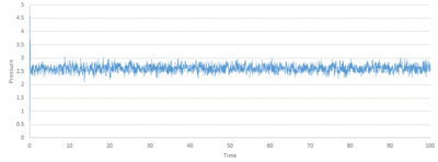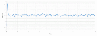
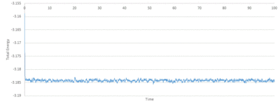
Looking at Figure 8-10 above, equilibrium is reached for all three, total energy, temperature and pressure. To investigate when the equilibrium is reached, a closer view of the graphs is needed:

‎Figure 11. Zoomed In: Total Energy against Time, for timestep=0.001

‎Figure 12. Zoomed In: Temperature against Time, for timestep=0.001

‎Figure 13. Zoomed In: Pressure against Time, for timestep=0.001

The average total energy at equilibrium is -3.184 and it is reached after 0.40 reduced units of time. The average temperature at equilibrium is around 1.24 and it is reached after 0.25 reduced units of time. The average pressure at equilibrium is around 2.5 reduced units and it is reached after approximately 0.30 reduced units of time.

Ranging the timestep as aforementioned gives representations of different accuracy of the physical properties. Shorter timesteps, run for less total time but increase the accuracy of the physical data. Looking at Figure 14 it is clear that all timesteps with the exception of 0.015 equilibrate giving a relatively constant total energy. The timestep of 0.015 does not reach equilibrium and it is therefore a bad choice of a timestep as it would not provide meaningful and representative results. Timestep of 0.0025 and 0.001 give roughly the same total energy and all larger timesteps provide deviation from it. Timestep of 0.0025 is the largest timestep to give representantive and accurate results. Using timestep of 0.0025 rather than a timestep of 0.001 provides longer time frames for simulation without affecting the results' accuracy. Timesteps of larger value such as 0.0075 and 0.01, whilst they equilibrate, they do at a higher total energy with greater fluctuations around the mean value.

‎Figure 14. Total Energy against Time, for timestep=0.001

JC: Good choice of timestep. The average total energy should not depend on the timestep so 0.01 and 0.0075 are not suitable.

Running Simulations Under Specific Conditions

TASK: Choose 5 temperatures (above the critical temperature $T^{*}=1.5$), and two pressures (you can get a good idea of what a reasonable pressure is in Lennard-Jones units by looking at the average pressure of your simulations from the last section). This gives ten phase points — five temperatures at each pressure. Create 10 copies of npt.in, and modify each to run a simulation at one of your chosen $(p,T)$ points. You should be able to use the results of the previous section to choose a timestep. Submit these ten jobs to the HPC portal. While you wait for them to finish, you should read the next section.

Looking at the average pressure as the section above, pressures of p=2.4 and p=2.6 were chosen. The timestep was set to 0.0025 as this proved to give the best results and the temperatures were set to 1.5, 2.0, 2.5, 3.0 and 3.5.

Thermostats and Barostats

TASK: We need to choose $\gamma$ so that the temperature is correct $T=\mathfrak{𝔗}$ if we multiply every velocity $\gamma$. We can write two equations:

$\frac{1}{2}\sum _i{m}_i{v}_i^2=\frac{3}{2}N{k}_{B}T$

$\frac{1}{2}\sum _i{m}_i{\left(\gamma v_i\right)}^2=\frac{3}{2}N{k}_B\mathfrak{𝔗}$

Solve these to determine $\gamma$.

To derive an equation for γ, first the velocity is multiplied by γ (ensures that fluctuations $\mathfrak{𝔗}$ are taken into account for each time step), then the two functions are added together:

$\frac{1}{2}\sum _i{m}_i{v}_i^2+\frac{1}{2}\sum _i{m}_i{\left(\gamma v_i\right)}^2=\frac{3}{2}N{k}_{B}T+\frac{3}{2}N{k}_B\mathfrak{𝔗}$

Which rearranges to:

$(1+{\gamma }^2)\frac{1}{2}\sum _i{m}_i{v}_i^2=(T+\mathfrak{𝔗})\frac{3}{2}N{k}_B$

$(1+{\gamma }^2)\sum _i{m}_i{v}_i^2=(T+\mathfrak{𝔗})3N{k}_B$

Since $\frac{1}{2}\sum _i{m}_i{v}_i^2=\frac{3}{2}N{k}_{B}T$ we can rewrite:

$(1+{\gamma }^2)3N{k}_{B}T=(T+\mathfrak{𝔗})3N{k}_B$

$(1+{\gamma }^2)T=(T+\mathfrak{𝔗})$

${\gamma }^2=\left(\frac{T+\mathfrak{𝔗}}{T}\right)-1$

${\gamma }^2=1+\left(\frac{\mathfrak{𝔗}}{T}\right)-1$

${\gamma }^2=\frac{\mathfrak{𝔗}}{T}$

$\gamma =\sqrt{\frac{\mathfrak{𝔗}}{T}}$

JC: Good.

Examining the Input Script

TASK: Use the manual page to find out the importance of the three numbers 100 1000 100000. How often will values of the temperature, etc., be sampled for the average? How many measurements contribute to the average? Looking to the following line, how much time will you simulate?

fix aves all ave/time 100 1000 100000 v_dens v_temp v_press v_dens2 v_temp2 v_press2
run 100000

The first number,

100

says that a sample should be calculated every 100 timesteps in order to get an average value. The second number,

1000 

says that this needs to be done 1000 1000 times. The average will thus cover

10,000

timesteps which is the third number.

Our simulation consisting of 10,000 atoms, we will have 1 average value for every 100th time step calculated contributing to the average.

The line

 run 100000

states that 100000 calculations should be run. Since our timestep is of 0.0025, this would be 250 reduced time units.

JC: The average will cover 100,000 timesteps, not 10,000.

Plotting the Equations of State

TASK: When your simulations have finished, download the log files as before. At the end of the log file, LAMMPS will output the values and errors for the pressure, temperature, and density $\left(\frac{N}{V}\right)$. Use software of your choice to plot the density as a function of temperature for both of the pressures that you simulated. Your graph(s) should include error bars in both the x and y directions. You should also include a line corresponding to the density predicted by the ideal gas law at that pressure. Is your simulated density lower or higher? Justify this. Does the discrepancy increase or decrease with pressure?

Temperatures chosen starting at the critical temperature of 1.5 reduced units and then at 2.0, 2.5, 3.0 and 3.5.

Pressures were chosen according to the average pressures acquired from the simulations above at p=2.4 and p=2.6.

The densities predicted by the ideal gas law at each of the pressures were calculated using the ideal gas law:

$PV=nRT$

which can be rewritten using density:

$PM=dRT$

which rearranges to:

$\frac{PM}{RT}=d$

P (pressure) was decided according to the parameter set (i.e. 2.4 or 2.6), M (molar mass) was set to 0.1, R is the universal gas constant and T (temperature) was also determined from the preset parameters.

JC: Remember that we are working in reduced units, you don't need the gas constant in this case (R = 1).

‎Figure 15. Density vs Temperature

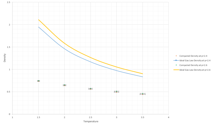
As seen from Figure 15, the simulated density is lower than the ideal gas density at each given temperature and pressure. To explain this, the approximations taken into account when the simulation were computed and when the ideal gas equation is used need to be investigated. The ideal gas assumes no particle-particle interaction which means that when two particles are in close proximity there is not effect on the potential energy. However this is not the case for the simulation used as the repulsive term in the Lennard Jones potential does indeed cause an increase in the potential energy when particles are close together, representing the repulsive interactions. This leads to particles of the simulation to be "repelled" from each other and to maintain a minimum distance between them. This leads to the density of the simulated system to therefore be lower than that of the ideal gas. Additionally, it is clear that for higher pressures (p=2.6) and for lower temperatures, the difference between the simulation and the ideal gas calculation. This is due to the fat that at higher temperatures and lower pressures the system behaves more like an ideal gas as it minimizes particle interaction and thus potential energy.

JC: Good, the ideal gas is a good approximation to a dilute gas (low pressure, high temperature) when inter particle interactions are less significant.

Heat Capacity Calculations

TASK: As in the last section, you need to run simulations at ten phase points. In this section, we will be in density-temperature $({\rho }^{*},T^{*})$ phase space, rather than pressure-temperature phase space. The two densities required at $0.2$ and $0.8$, and the temperature range is $2.0,2.2,2.4,2.6,2.8$. Plot $C_V/V$ as a function of temperature, where $V$ is the volume of the simulation cell, for both of your densities (on the same graph). Is the trend the one you would expect? Attach an example of one of your input scripts to your report.

‎Figure 16.Heat Capacity vs Temperature at Densities 0.2, 0.8 and 1.2

As seen from the equation below, specific heat capacity is temperature dependent.

$C_V=\frac{\partial E}{\partial T}$

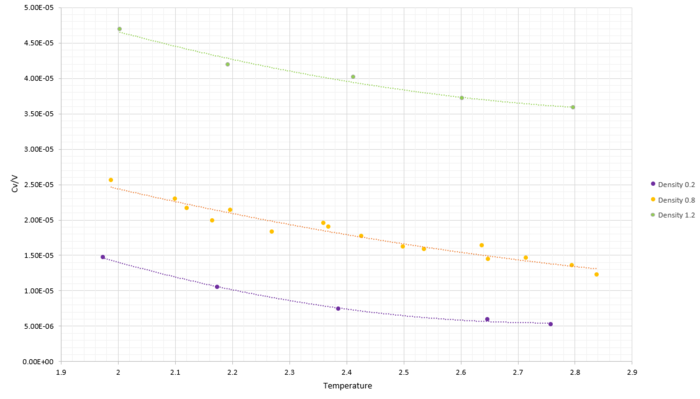
Looking at the heat capacities per volume against temperature, it seems to follow a fourth order polynomial fit. A higher density, namely of 1.2 was tested to see if the trend exists regardless of density. After this was confirmed an increased number of temperature samples was taken to see whether it truly fitted through a fourth order polynomial. Increase the temperature samples showed that the relationship of heat capacity per volume against temperature is not a fourth order polynomial. Thus a curve was fitted through, corresponding to the inverse relationship between increase in temperature and increase in heat capacity per volume, as explained below.

The heat capacity shows how easy it is to excite the system to a higher energy state. For a gas, the molar heat capacity C is the heat required to increase the temperature of 1 mole of gas by 1 K. Heat capacity is an extensive property and it is expected to increase with the number of atoms present. The heat capacity per volume is thus expected to increase when the number of molecules per unit volume increases, which is clearly shown by Figure 16 by the increase in heat capacity with an increase in density.

For real gases, heat capacities increase with an increase in temperature. The trend observed here is opposite from what expected. Heat capacity per unit volume decreases with temperature. To explain this, the electronic structure for the material at study is required. However a general explanation is based on the assumption that energy levels are more closely packed with increasing energy. This increasing energy can be presented by the increase in temperature. If the energy states are more closely packed with increasing temperature then it is easier to excite the system to a higher energy, giving an inverse relationship between heat capacity and temperature.

Another possible explanation is based on the vibrational energy of the system. At higher temperatures, the system has more vibrational energy. As a result excitation is easier making heat capacity per unit volume to decrease with increasing temperature.

Input File for density of 0.2, temperature of 2.4: File:R0224.txt

JC: Give the equations for the functions which you have fit to the data. Remember that these simulations are classical so there is no electronic structure in these simulations, but the heat capacity can be related to the density of energy states. There is also no vibrational energy in these simulations are the system only contains spherical particles.

Structural Properties and the Radial Distribution Function

TASK: perform simulations of the Lennard-Jones system in the three phases. When each is complete, download the trajectory and calculate $g(r)$ and $\int g(r)\mathrm{d}r$. Plot the RDFs for the three systems on the same axes, and attach a copy to your report. Discuss qualitatively the differences between the three RDFs, and what this tells you about the structure of the system in each phase. In the solid case, illustrate which lattice sites the first three peaks correspond to. What is the lattice spacing? What is the coordination number for each of the first three peaks?

Looking at the phase diagram of the Lennard-Jones system the density value chosen for liquid was chosen as 0.8, density for solid was chosen as 1.5 and for vapour 0.01 with temperature kept constant at T=1.2. Calculating the Radial Distribution Function (RDF) using VMD and plotting it for each of the three phases against r gives Figure 17 below:

Figure 17: Radial distribution function for vapour, liquid, solid and gas

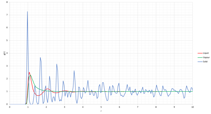
The RDF represents the atom density around any particle in the system. When the RDF is at 0, it means that there are no neighboring atoms in close proximity. This can be explained by the Lennard-Jones potential which was used to calculate the inter-atomic interactions in the system. For small inter-atomic distances, the potential energy is really high, making configuration with inter-atomic distance smaller than 0.9 energetically unfavorable.

The vapour RDF (green) shows a broad peak at inter-atomic distance of 1.125 and then decreases to a constant value of 1. This behavior is explained by the lack of order in the vapour phase which means that odds of finding another atom is low, averaging the density to a constant value.

The liquid RDF (red) shows three broad peaks of decreasing intensity before plateauing. The difference from the vapour is due to an increased degree of order, yet due to some extend of disorder and the atoms being able to move freely compared to each other, it still averages to a single density. Long range order is thus not observed.

The solid RDF (blue) shows sharp fluctuations of decreasing intensity throughout the inter-atomic distances studied. This can be explained by a high degree of order (both short and long range) in the fcc solid lattice. The decrease in peak intensity is due to the vibrational motion of the particles in the solid stucture. The peaks of the solid RDF correspond to coordinates of points on the fcc lattice. They come at regular distance intervals, which is the length of the unit cell.

Figure 18: Radial distribution function for solid, zoomed-in in first region

FCC lattice (three nearest coordination sites of central atom labeled A, B and C)

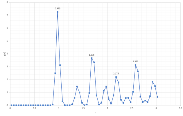
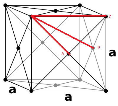
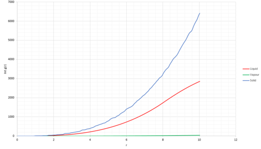
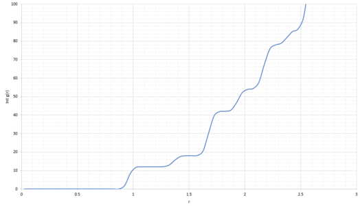
Lattice points A, B and C correspond to the coordinates of the first three peaks (Figure 18) and follow coordination numbers taken from the "long" plateaus in the integral graph (Figure 20).

From the integral of the radial distribution function, seen in Figure 19 and 20 below, shows how many atoms are interacting in the same way, at a specific distance r. For example, looking at the solid integral, Figure 20, at distance 0.975 there are 12 atoms interacting, at 1.675 there were 42 and at 2.175 there were 77.

Figure 19: Integral of RDF

Figure 20: Integral of RDF for solid, zoomed-in in first region

JC: The coordination numbers are cumulative, the second peak represents 6 atoms (18 - 12) and the third peak represents 24 (42 - 18), can you see that these numbers make sense by looking at a diagram of an fcc lattice? Did you calculate the lattice parameter?

Dynamical Properties and the Diffusion Coefficient

Mean Squared Displacement

TASK: Make a plot for each of your simulations (solid, liquid, and gas), showing the mean squared displacement (the "total" MSD) as a function of timestep. Are these as you would expect? Estimate $D$ in each case. Be careful with the units! Repeat this procedure for the MSD data that you were given from the one million atom simulations.

Figure 21: MSD against Timestep for Liquid of 8000 Atoms

Figure 22: MSD against Timestep for Vapour of 8000 Atoms

Figure 23: MSD against Timestep for Solid of 32,000 Atoms

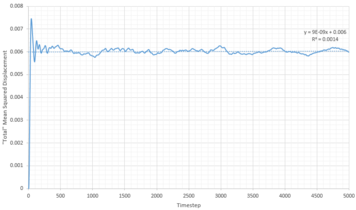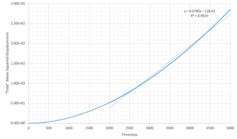
The diffusion coefficients were calculated using:

$D=\frac{1}{6}\frac{\partial ⟨r^2\left(t\right)⟩}{\partial t}$

$\frac{\partial ⟨r^2\left(t\right)⟩}{\partial t}$ gives the gradient of the MSD against timestep plots (Figures 21-23). However this gradient does not have the correct units as the plots are in timestep and therefore the gradient is divided by 0.002. To get the diffusion coefficient the above equation is used and thus it is divided by six. This is summarized by Figure 24 below:

Figure 24: Gradient to Diffusion Coefficient

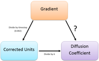
This results in diffusion coefficients according to:

Diffusion Coefficient Summary for 8K/32K Atom System

Phase	Gradient	Diffusion Coefficient
Liquid	0.001	0.0833
Vapour	0.0782	6.52
Solid	9 x 10 -9	7.5 x 10 -7

The "total" mean standard displacement against timestep was also repeated for the files of 1,000,000 atoms and are summarized below (Figures 25-27).

Figure 25: MSD against Timestep for Liquid of 1,000,000 Atoms

Figure 26: MSD against Timestep for Vapour of 1,000,000 Atoms

Figure 27: MSD against Timestep for Solid of 1,000,000 Atoms

Diffusion Coefficient Summary for 1M Atom System

Phase	Gradient	Diffusion Coefficient
Liquid	0.001	0.0833
Vapour	0.037	3.083
Solid	5 x 10 -8	4.17 x 10 -6

The 8K-atom system and the 1M-atom system show similar trends in the graphs. This suggests that a smaller number of atoms such as 8,000 can be used to simulate a real physical system consisting of millions of atoms.

Looking at the liquid phases (Figures 21 and 25) there is a linear relationship between the mean squared displacement and increasing timesteps. This is as expected, as atoms move and collide randomly due the nature of particles suspended in a fluid known as pedesis (or Brownian motion).

Looking at the vapor phases (Figures 22 and 26), initially a quadratic behavior is observed, but then the relationship is linear (after 2,500 timesteps). this shows that initially atoms do not participate in frequent collision, but instead move free through space due to large inter-atomic distance. This allows their movement (i.e. displacement) to increase linearly with time. Taking the squared displacement which is used plot the graph gives a quadratic nature to the curve. The quadratic region however is not of interest as we only focus on the system's properties once equilibration has been achieved and atoms collide. The gradient of the vapor phase was thus calculated using a linear fit on the region above 2,500 timesteps. After the 2,500th timestep the same trend as for liquids is observed also due to pedesis.

Diffusion coefficient for vapor however were greater than those for liquid. This is also as expected as particles in the gas phase move a lot more freely that those in a liquid due to the greater number of intermolecular interactions in liquid and thus greater degree of ordering compared to gas.

Looking at the solid phases (Figures 23 and 27), the MSD increases rapidly and then plateaus (with some fluctuations) for the remainder of the simulation giving a very low diffusion coefficient compared to liquids and gases which comes in agreement with the highly order structure of solids, and the inability of atoms to move freely.

JC: Good explanation of the shape of the vapour phase MSD and the ballistic regime. Make sure that you only fit the linear part of the MSD to get the diffusion coefficient.

Velocity Autocorrelation Function

TASK: In the theoretical section at the beginning, the equation for the evolution of the position of a 1D harmonic oscillator as a function of time was given. Using this, evaluate the normalised velocity autocorrelation function for a 1D harmonic oscillator (it is analytic!):

$C\left(\tau \right)=\frac{\underset{-\mathrm{\infty }}{\overset{\mathrm{\infty }}{\int }}v\left(t\right)v(t+\tau )\mathrm{d}t}{\underset{-\mathrm{\infty }}{\overset{\mathrm{\infty }}{\int }}{v}^2\left(t\right)\mathrm{d}t}$

Be sure to show your working in your writeup. On the same graph, with x range 0 to 500, plot $C\left(\tau \right)$ with $\omega =1/2\pi$ and the VACFs from your liquid and solid simulations. What do the minima in the VACFs for the liquid and solid system represent? Discuss the origin of the differences between the liquid and solid VACFs. The harmonic oscillator VACF is very different to the Lennard Jones solid and liquid. Why is this? Attach a copy of your plot to your writeup.

From the equation of the position of the harmonic oscillator:

$x\left(t\right)=A\cos (\omega t+\varphi )$

Taking the derivative gives the velocity:

$v\left(t\right)=\frac{\text{d}x\left(t\right)}{\text{d}t}=-A\omega \sin (\omega t+\varphi )$

$v(t+\tau )=-A\omega \sin (\omega (t+\tau )+\varphi )$

Substituting into original eqn:

$$\begin{gathered} C(\tau )=\frac{\underset{-\mathrm{\infty }}{\overset{\mathrm{\infty }}{\int }}(-A\omega \sin (\omega t+\varphi ))\cdot (-A\omega \sin (\omega (t+\tau )+\varphi )\text{d}t}{\underset{-\mathrm{\infty }}{\overset{\mathrm{\infty }}{\int }}(A^2{\omega }^2 \\ si{n}^2(\omega t+\varphi ))\text{d}t} \end{gathered}$$

$=\frac{\underset{-\mathrm{\infty }}{\overset{\mathrm{\infty }}{\int }}(\sin (\omega t+\varphi ))\cdot (\sin (\omega (t+\tau )+\varphi )\text{d}t}{\underset{-\mathrm{\infty }}{\overset{\mathrm{\infty }}{\int }}{\sin }^2(\omega t+\varphi )\text{d}t}$

Since $sin(a+b)=sin(a)cos(b)+sin(b)cos(a)$

It can be written:

$C(\tau )=\frac{\underset{-\mathrm{\infty }}{\overset{\mathrm{\infty }}{\int }}(sin(\omega t+\varphi ))[sin(\omega t+\varphi )cos(\omega \tau )+cos(\omega t+\varphi )sin(\omega \tau )]\text{d}t}{\underset{-\mathrm{\infty }}{\overset{\mathrm{\infty }}{\int }}si{n}^2(\omega t+\varphi )\text{d}t}$

$=\frac{\underset{-\mathrm{\infty }}{\overset{\mathrm{\infty }}{\int }}si{n}^2(\omega t+\varphi )cos(\omega \tau )+sin(\omega t+\varphi )cos(\omega t+\varphi )sin(\omega \tau )\text{d}t}{\underset{-\mathrm{\infty }}{\overset{\mathrm{\infty }}{\int }}si{n}^2(\omega t+\varphi )\text{d}t}$

$=\frac{cos(\omega \tau )\underset{-\mathrm{\infty }}{\overset{\mathrm{\infty }}{\int }}si{n}^2(\omega t+\varphi )\text{d}t+sin(\omega \tau )\underset{-\mathrm{\infty }}{\overset{\mathrm{\infty }}{\int }}sin(\omega t+\varphi )cos(\omega t+\varphi )\text{d}t}{\underset{-\mathrm{\infty }}{\overset{\mathrm{\infty }}{\int }}si{n}^2(\omega t+\varphi )\text{d}t}$

$=cos(\omega \tau )+\frac{sin(\omega \tau )\underset{-\mathrm{\infty }}{\overset{\mathrm{\infty }}{\int }}sin(\omega t+\varphi )cos(\omega t+\varphi )\text{d}t}{\underset{-\mathrm{\infty }}{\overset{\mathrm{\infty }}{\int }}si{n}^2(\omega t+\varphi )\text{d}t}$

Integrating from $-\mathrm{\infty }$ to $\mathrm{\infty }$ means that:

$\underset{-\mathrm{\infty }}{\overset{\mathrm{\infty }}{\int }}sin(\omega t+\varphi )cos(\omega t+\varphi )\text{d}t=0$

Therefore:

$C(\tau )=cos(\omega \tau )$

JC: Correct.

Figure 28. Velocity against Time Step for Liquid and Solid VACF and Harmonic Oscillator

Looking at Figure 28, the solid shows more intense minima that also last for a longer timestep period compared to the liquid. This relates to the RDF of the liquid and solid that were seen in previous sections. In the solid system the atoms are in fixed position, and are ordered in both long and short range. Upon collision, the almost stationary atoms in the solid system change velocity greatly. For the liquid phase whilst short range order exists, long range doesn't. Collisions with neighboring atoms in the liquid result in a relatively large change in velocity in the short term (therefore a minimum is observed) but due to the lack of ordering in longer range, there is no change in velocity in the long run.

The VACF of both liquid and solid eventually goes to zero. This can be explained by repeating collisions which make velocity of atoms to become decorrelated over time as the collisions cause velocity in different directions which cancels the overall velocity to cancel out. The Harmonic Oscillator approxiamtiondoes not account for any collisions, therefore velocity does not get "decorrelated" over time and thus it never converges.

JC: What do you mean "there is no change in velocity in the long run"? The velocities in the solid and liquid decorrelate eventually as the VACF decays to zero. Make sure you don't get confused between the RDF and VACF.

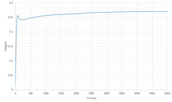
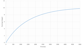
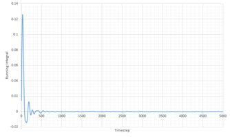
TASK: Use the trapezium rule to approximate the integral under the velocity autocorrelation function for the solid, liquid, and gas, and use these values to estimate $D$ in each case. You should make a plot of the running integral in each case. Are they as you expect? Repeat this procedure for the VACF data that you were given from the one million atom simulations. What do you think is the largest source of error in your estimates of D from the VACF?

The trapezium rule is defined as:

$\underset{a}{\overset{b}{\int }}f(x)dx\approx (b-a)\left[\frac{f(a)+f(b)}{2}\right]$

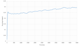
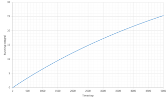
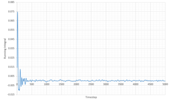
The diffusion coefficients, D, were caclulated using the running integral of the VACF, following conversion to reduced time units. D was calculated using:

$D=\frac{1}{3}\underset{0}{\overset{\mathrm{\infty }}{\int }}\mathrm{d}\tau ⟨\mathbf{v}\left(0\right)\cdot \mathbf{v}\left(\tau \right)⟩$

Figure 29: Int. VACF against Timestep for Liquid of 8000 Atoms

Figure 30: Int. VACF against Timestep for Vapour of 8000 Atoms

Figure 31: Int. VACF against Timestep for Solid of 32,000 Atoms

Diffusion Coefficient Summary for 8K/32K Atom Systems

Phase	Total Summed Integral	Diffusion Coefficient
Liquid	0.2940	0.0979
Vapour	25.34	8.45
Solid	-1.8 x 10-4	-5.91 x 10 -5

Figure 32: Int. VACF against Timestep for Liquid of 1M Atoms

Figure 33: Int. VACF against Timestep for Vapour of 1M Atoms

Figure 34: Int. VACF against Timestep for Solid of 1M Atoms

Diffusion Coefficient Summary for 1M Atom Systems

Phase	Total Summed Integral	Diffusion Coefficient
Liquid	0.2703	0.0901
Vapour	9.806	3.269
Solid	1.36 x 10-4	4.548 x 10 -5

The diffusion coefficients follow the expected trend, of smallest D for the solid and largest for the gas. Qualitatively the trend is comparable to that generated from the MSD calculations above. However the quantitative values are very different. Comparing the diffusion coefficient using VACF, it is obvious that the smallest difference in D between the system sizes is that of the liquid system, indicating that these simulations work best for liquids.

It is worth noting that a large amount of error is expected due to the use of the trapezium rule. Additionally error is present in all our calculations because of the system sizes used. This is especially true for the solid and vapor phases as large discrepancies can be seen between the diffusion coefficients of the two systems. Additionally some error can be attributed to the classical approach of molecular dynamics which doesn't take into account the quantum mechanics such as the zero point energy.

JC: Calculating D from the VACF also relies on the integral of the VACF reaching a plateau within the simulation time, is this valid for these simulations?