Talk:Mod:JMW114

JC: General comments: All tasks attempted, but a few mistakes, especially in some of the early sections. Make sure you properly understand the background theory to these tasks and check that your results make sense and are what you would expect.

Third year simulation experiment : Molecular Dynamics Simulation

Running your first simulation

• All of the simulations that are run in this experiment are performed on the Imperial College High Performance Compution systems (HPC).
• Five simulations were run each with a different timestep varying from 0.001 to 0.015

Introduction to Molecular Dynamics Simulation

• TASK 1: Open the file HO.xls. In it, the velocity-Verlet algorithm is used to model the behaviour of a classical harmonic oscillator. Complete the three columns "ANALYTICAL", "ERROR", and "ENERGY": "ANALYTICAL" should contain the value of the classical solution for the position at time , "ERROR" should contain the absolute difference between "ANALYTICAL" and the velocity-Verlet solution (i.e. ERROR should always be positive -- make sure you leave the half step rows blank!), and "ENERGY" should contain the total energy of the oscillator for the velocity-Verlet solution. Remember that the position of a classical harmonic oscillator is given by (the values of $A$, $\omega$, and $\varphi$ are worked out for you in the sheet).
  • Part 1: Analytical: Equation used is $x(t)=Acos(\omega t+\varphi )$ which translates into the excel document as =$H$2*(COS(($H$3*B6)+$H$1)), with each of the letters representing each of the parts of the equation respectively
  • Part 2: Error: Absolute value taken of the classical atom position subtracted from the velocity-Verlet solution atom position using the excel equation =ABS(F6-C6)
  • Part 3: Energy: Total energy of the oscillator calculated by adding the kinetic energy and potential energy ($E=\frac{1}{2}m{v}^2+mgx$) using the velocity-Verlet atom position solutions, this translated to the excel equation =(0.5*($B$3*(D6^2)))+($B$3*9.81*C6)
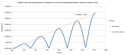
• TASK 2:

  

  Figure 1: Diagram to show the function plotted to follow the error maxima.

  For the default timestep value, 0.1, estimate the positions of the maxima in the ERROR column as a function of time. Make a plot showing these values as a function of time, and fit an appropriate function to the data.
  • Using the previous calculations a plot of error vs time was used to find out the region where the error maxima were. The data was then analysed to find the exact points where the maxima were seen and the time and error value recorded. These were then plotted on the same graph and a line of best fit plotted. The equation of the line of best fit was $y=0.0004x-7\text{x}10^{-5}$.

JC: Why does the error oscillate?

• TASK 3: Experiment with different values of the timestep. What sort of a timestep do you need to use to ensure that the total energy does not change by more than 1% over the course of your "simulation"? Why do you think it is important to monitor the total energy of a physical system when modelling its behaviour numerically?
  • Part 1: The maximum timestep is 0.2. If the timestep is increased any further the energy oscillated by more than 1%.
  • Part 2: It is important to monitor the total energy of a physical system when modelling its behaviour numerically as should no external forces be present in the simulation we would expect the total energy of the system to remain constant. The reason for doing numerical solutions is usually due to an analytical solution not being possible.

JC: Good choice of timestep.

• TASK 4: For a single Lennard-Jones interaction, $\varphi \left(r\right)=4ϵ(\frac{{\sigma }^{12}}{r^{12}}-\frac{{\sigma }^6}{r^6})$, find the separation, $r_0$, at which the potential energy is zero. What is the force at this separation? Find the equilibrium separation, $r_{eq}$, and work out the well depth ($\varphi \left(r_{eq}\right)$). Evaluate the integrals $\underset{2\sigma }{\overset{\mathrm{\infty }}{\int }}\varphi \left(r\right)\mathrm{d}r$, $\underset{2.5\sigma }{\overset{\mathrm{\infty }}{\int }}\varphi \left(r\right)\mathrm{d}r$, and $\underset{3\sigma }{\overset{\mathrm{\infty }}{\int }}\varphi \left(r\right)\mathrm{d}r$ when $\sigma =ϵ=1.0$.
  • Part 1: The $\varphi \left(r\right)=4ϵ(\frac{{\sigma }^{12}}{r^{12}}-\frac{{\sigma }^6}{r^6})$ equation was used to calculate the separation, $r_0$, at which the potential energy was zero. This was done by equating $\varphi \left(r\right)=0$ and using the fact that $\sigma =ϵ=1.0$, this gave the equation $\frac{r_0^6}{r_0^{12}}=4$ which in turn meant that $r_0=0.7937$
  • Part 2: The force at $r_0=0.7937$ was calculated by differentiating the equation $\varphi \left(r\right)=4ϵ(\frac{{\sigma }^{12}}{r^{12}}-\frac{{\sigma }^6}{r^6})$, to get ${\mathbf{F}}_i=-\frac{\mathrm{d}U\left({\mathbf{r}}^N\right)}{\mathrm{d}{\mathbf{r}}_i}$. This gave ${\text{F}}_i=4ϵ(\frac{12{\sigma }^{12}}{r_0^{13}}-\frac{6{\sigma }^6}{r^7})$. The values of $\sigma =ϵ=1.0$ were subbed in and the calculated distance from part 1, $r_0=0.7937$, was also subbed in, when calculated this gave ${\text{F}}_i=846.67$.
  • Part 3: The equilibrium seperation was found using the fact that at $r_{eq}$, ${\text{F}}_i=0$, therefore using the same differential as in the previous step the equation to be solved is found to be $0=4ϵ(\frac{12{\sigma }^{12}}{r_{eq}^{13}}-\frac{6{\sigma }^6}{r_{eq}^7})$, this gave $r_{eq}=1.122462$
  • Part 4: The well depth was found using the initial equation $\varphi \left(r_{eq}\right)=4ϵ(\frac{{\sigma }^{12}}{r^{12}}-\frac{{\sigma }^6}{r^6})$ , subbing in the equilibrium distance found in the previous part, $r_{eq}=1.122462$, and $\sigma =ϵ=1.0$, the answer was calculated to be $\varphi \left(r_{eq}\right)=-1$
  • Part 5: The integrals were evaluated by using the equations $\underset{2\sigma }{\overset{\mathrm{\infty }}{\int }}\varphi \left(r\right)\mathrm{d}r$ and $\varphi \left(r\right)=4ϵ(\frac{{\sigma }^{12}}{r^{12}}-\frac{{\sigma }^6}{r^6})$ to form the equation $\underset{x\sigma }{\overset{\mathrm{\infty }}{\int }}4ϵ(\frac{{\sigma }^{12}}{r^{12}}-\frac{{\sigma }^6}{r^6}).dr$. The values of $\sigma =1$ and $ϵ=1$ were subsituted into the equation and it was integrated to give $4_{x_{}}^{{}^{\mathrm{\infty }}}(\frac{0.2}{r^5}-\frac{1}{11r^{11}})$, when subbing in infinite, the first term always became zero and the second term varied depending on the value of x. When $x=2$ the integral output was 0.025, when $x=2.5$ the integral output was 0.0082, and when $x=3$ the integral output was 0.0033.

JC: Give analytical answers to the first questions rather than numerical values: r0 = sigma (=1), F=24*epsilon/sigma, well depth = epsilon. Integrals are correct.

• TASK 5: Estimate the number of water molecules in 1ml of water under standard conditions. Estimate the volume of 10000 water molecules under standard conditions.
  • Part 1: Under standard conditions, water has a density of 1g/ml and its molecular mass is 18.01528g/mol, we can therefore calculate that 1g and thus 1ml contains 3.34 x 10²² molecules by dividing the Avogadros constant by the molar mass.
  • Part 2: Using the molar mass, we can calculate that 1 molecule is equivalent to 2.99 x 10^-23 ml, and therefore 10,000 molecules would be equivalent to 2.99 x 10^-19 ml.

JC: Correct.

• TASK 6: Consider an atom at position $(0.5,0.5,0.5)$ in a cubic simulation box which runs from $(0,0,0)$ to $(1,1,1)$. In a single timestep, it moves along the vector $(0.7,0.6,0.2)$. At what point does it end up, after the periodic boundary conditions have been applied?
  • An atom at position (0.5,0.5,0.5) moves to hit the x boundary which causes the x velocity to change in the opposite direction whilst the others remain the same. Later, the atom bounces of the u wall, which causes the y velocity to change direction. As for the z velocity it does not ever change within this timestep. This results in the following:

    

    Figure 2: Diagrams to show the movement of the atom along the vector, in the single timestep the atom never hits the z boundary but hits both the x and then the y causing the velocitys to change in the opposite direction in both these cases (essentially the atom then bounces back), finishing at position (0.8,0.9,0.7).

JC: The atom doesn't bounce off the wall, but instead passes through the wall and re-enters the box from the opposite side, so the final position should be (0.2, 0.1, 0.7)).

• TASK 7: The Lennard-Jones parameters for argon are $$\begin{gathered} \sigma =0.34\mathrm{n}\mathrm{m},ϵ \\ / \\ {k}_B=120\mathrm{K} \end{gathered}$$. If the LJ cutoff is $r^{*}=3.2$, what is it in real units? What is the well depth in $$\begin{gathered} {\mathrm{k}\mathrm{J} \\ \mathrm{m}\mathrm{o}\mathrm{l}}^{-1} \end{gathered}$$? What is the reduced temperature $T^{*}=1.5$ in real units?
  • Part 1: Using the equation,$r^{*}=\frac{r}{\sigma }$,we can convert the LJ cutoff,$r^{*}=3.2$, to the real units by subbing in the value of $\sigma$. This gives the answer $r=1.088\mathrm{n}\mathrm{m}$
  • Part 2: We can calculate the well depth in real units by substituting in the values of $ϵ$, $\sigma$ and $r$ given/calculated above into the equation $\varphi \left(r\right)=4ϵ(\frac{{\sigma }^{12}}{r^{12}}-\frac{{\sigma }^6}{r^6})$. This gives the well depth $$\begin{gathered} E=-6.16\text{x}10^{-27}{\mathrm{k}\mathrm{J} \\ \mathrm{m}\mathrm{o}\mathrm{l}}^{-1} \end{gathered}$$
  • Part 3: Using the equation,$T^{*}=\frac{k_{B}T}{ϵ}$, we can convert the reduced temperature,$T^{*}=1.5$, to real units by subbing in the value of ${k}_B/ϵ$,$T=180\mathrm{K}$

JC: The well depth is epsilon, so you just need to convert this into kJ mol-1, part 1 and 3 are correct.

Equilibration

• TASK 1: Why do you think giving atoms random starting coordinates causes problems in simulations? Hint: what happens if two atoms happen to be generated close together?
  • Giving the atoms random starting coordinated causes problems in simulations due to two main reasons. First, if we consider a situation similar to the one we are simulating, two particles in a box, we would expect the particles to spread to opposite sides of the box due to repulsive forces, this of course does not happen when the atoms are given random starting coordinates and would result in the total energy being increased. Secondly, random coordinates can lead to the atoms being placed in positions where they overlap, and this is physically impossible.

JC: If particles overlap the high repulsive forces can cause the simulation to crash.

• TASK 2: Satisfy yourself that this lattice spacing corresponds to a number density of lattice points of 0.8. Consider instead a face-centred cubic lattice with a lattice point number density of 1.2. What is the side length of the cubic unit cell?
  • Part 1: By multiplying the x,y and z coordinates provided we can calculate the volume each atom occupies i.e. 1.07722³ . By then doing the reciprocal of this we can find out the quantity of atoms per unit volume (a.k.a the number density). $NumberDensity=\frac{1}{1.07722^3}=0.7999$
  • Part 2: Using the lattice point number density, 1.2, we can calculate the side length of the cubic unit cell by doing the opposite of the above. However this time we must multiply the reciprocal by 3 to account for each unit cell having $6\text{x}\frac{1}{2}$ atoms in it. $SideLengthofUnitCell=\sqrt[3]{\frac{1}{1.2}\text{x}3}=1.36$
• TASK 3: Consider again the face-centred cubic lattice from the previous task. How many atoms would be created by the create_atoms command if you had defined that lattice instead?
  • By considering the face-centred cubic lattice we once again consider, as above that the unit cell now contains 3 atoms instead of 1. Thus if we used the create_atoms command having defined the new lattice type we would expect 3000 (3 x 1000) atoms to be created.

JC: The fcc unit cell has 4 atoms in it, not 3.

• TASK 4: Using the LAMMPS manual, find the purpose of the following commands in the input script:

mass 1 1.0
pair_style lj/cut 3.0
pair_coeff * * 1.0 1.0

• • mass 1 1.0, general form of the function = mass I Value, this function allows the mass of a certain type of atom (I) to be set to at a certain value (Value)
  • pair_style lj/cut 3.0, general form of the function = pair_style style args, pair_style where 'style' is lj/cut computes the standard lennard-jones potential with the argument (args) as the cut off
  • pair_coeff * * 1.0 1.0, general form of the function = pair_coeff I J args, the function allows us to set the pairwise force field coefficients (args) for one or more pairs of atom types (I,J). The number and meaning of the coefficients depends on the pair style.

JC: What are the pair coefficients for a Lennard Jones forcefield?

• TASK 5: Given that we are specifying ${\mathbf{x}}_i\left(0\right)$ and ${\mathbf{v}}_i\left(0\right)$, which integration algorithm are we going to use?
  • As we are using a canonical system where we want to generate position and velocities using time integration the most suitable integration algorithm is the fix nvt command. More specifically we would most likely use the full command fix 1 all nvt temp x x iso y y, where x is the start/end temperature respectively and y is the start/end pressure. The manual definition of this command is, these commands perform time integration on Nose-Hoover style non-Hamiltonian equations of motion which are designed to generate positions and velocities sampled from the canonical (nvt) ensembles. This updates the position and velocity for atoms in the group each timestep.

• TASK 6: Look at the lines below.

### SPECIFY TIMESTEP ###
variable timestep equal 0.001
variable n_steps equal floor(100/${timestep})
variable n_steps equal floor(100/0.001)
timestep ${timestep}
timestep 0.001

### RUN SIMULATION ###
run ${n_steps}
run 100000

The second line (starting "variable timestep...") tells LAMMPS that if it encounters the text ${timestep} on a subsequent line, it should replace it by the value given. In this case, the value ${timestep} is always replaced by 0.001. In light of this, what do you think the purpose of these lines is? Why not just write:

timestep 0.001
run 100000

• • The code is written as such so as to generalise the formula, so as to allow the user to easily change the timestep without having to manually change it each time.
• TASK 7: make plots of the energy, temperature, and pressure, against time for the 0.001 timestep experiment (attach a picture to your report). Does the simulation reach equilibrium? How long does this take? When you have done this, make a single plot which shows the energy versus time for all of the timesteps (again, attach a picture to your report). Choosing a timestep is a balancing act: the shorter the timestep, the more accurately the results of your simulation will reflect the physical reality; short timesteps, however, mean that the same number of simulation steps cover a shorter amount of actual time, and this is very unhelpful if the process you want to study requires observation over a long time. Of the five timesteps that you used, which is the largest to give acceptable results? Which one of the five is a particularly bad choice? Why?
  • Part 1: The graphs can be analysed easily, the minute differences in temperature and pressure mean we can come to the conclusion that equilibrium is reached after 0.3 seconds even though we would expect energy to be conserved and remain constant at equilibrium. These small fluctuations can be put down to the numerical error of the solution.

JC: We are using reduced units, time is not in seconds.

Figure 3: Graphs to show how energy, temperature and pressure vary with time.

• • Part 2: From the graph we can see that the accuracy of the 0.001 and 0.0025 timesteps are very similar, this is closely followed by 0.0075 and 0.01. I would therefore suggest that the ideal timestep to use when doing further simulations would be 0.0025. The 0.015 timestep is a particularly bad choice as the recorded values are completely different to those seen at the higher, more accurate timesteps.

Figure 4: Graph to show how varying the timestep effects the energy recorded at a certain time.

JC: Good choice of timestep. The average total energy should not depend on the timestep and 0.0025 is the largest timestep which agrees with this.

Running Simulations Under Specific Conditions

• TASK 1: Choose 5 temperatures (above the critical temperature $T^{*}=1.5$), and two pressures (you can get a good idea of what a reasonable pressure is in Lennard-Jones units by looking at the average pressure of your simulations from the last section). This gives ten phase points — five temperatures at each pressure. Create 10 copies of npt.in, and modify each to run a simulation at one of your chosen $(p,T)$ points. You should be able to use the results of the previous section to choose a timestep. Submit these ten jobs to the HPC portal. While you wait for them to finish, you should read the next section.
  • Simulations were undertaken at timestep 0.0025. The temperatures chosen were 2,10,20,30, and 40 and recorded at pressures of 2 and 10.
• TASK 2: We need to choose $\gamma$ so that the temperature is correct $T=\mathfrak{𝔗}$ if we multiply every velocity $\gamma$. We can write two equations. Solve these to determine $\gamma$.

$E_K=\frac{3}{2}N{k}_{B}T$ $\frac{1}{2}\sum _i{m}_i{v}_i^2=\frac{3}{2}N{k}_{B}T$

• • To solve this we need to essentially equate ${\gamma }^{2}T=\mathfrak{𝔗}$. Using the above equations we get ${\gamma }^{2}T=\frac{{\gamma }^2}{3N{k}_B}\sum _i{m}_i{v}_i^2=\mathfrak{𝔗}$. This can then be equated to get $\gamma =\sqrt{\frac{3N{k}_B\mathrm{\Im }}{\sum _i{m}_i{v}_{{}^{2}i}}}$.

JC: Use gamma to scale the velocities so that the target temperature is achieved, gamma should be $\gamma =\sqrt{\frac{\mathfrak{𝔗}}{T}}$.

• TASK 3: Use the manual page to find out the importance of the three numbers 100 1000 100000. How often will values of the temperature, etc., be sampled for the average? How many measurements contribute to the average? Looking to the following line, how much time will you simulate?
  • Part 1: The fix/ave time command,fix aves all ave/time 100 1000 100000 v_dens v_temp v_press v_dens2 v_temp2 v_press2, has the general form: fix ID group-ID ave/time Nevery Nrepeat Nfreq value1 value2 ... keyword args ... , from this we can see that the three values, 100, 1000 and 100000 correspond to Nevery, Nrepeat and Nfreq respectively. Nevery in this case means use input values every 100 timesteps. Nrepeat means use the input values for calculating averages 1000 times. Nfreq means calculate averages every 100000 timesteps.
  • Part 2: The following line, run 100000, indicates that the simulation should simulate 100000 timesteps where each timestep is 0.0025 which is equivalent to 250 seconds.

• TASK 4: When your simulations have finished, download the log files as before. At the end of the log file, LAMMPS will output the values and errors for the pressure, temperature, and density $\left(\frac{N}{V}\right)$. Use software of your choice to plot the density as a function of temperature for both of the pressures that you simulated. Your graph(s) should include error bars in both the x and y directions. You should also include a line corresponding to the density predicted by the ideal gas law at that pressure. Is your simulated density lower or higher? Justify this. Does the discrepancy increase or decrease with pressure?

Figure 5: Graph to show how simulation densities compare to those of the ideal gas law. The simulated densitys are higher in both cases, which in turn means that they did not expand as much as the densitys produced by the ideal gas law, the discrepancy as expected increase with pressure. The line of best fit can be seen in all cases to be 1/x which is in line with the ideal gas law,as pV = nRT we would expect T = a constant multiplied by the reciprocal of density.

JC: Is this what you would expect? The ideal gas has no interactions and so should have a higher density than the simulation results since in the simulations particles repel each other.

Calculating Heat Capacities Using Statistical Physics

• TASK 1: As in the last section, you need to run simulations at ten phase points. In this section, we will be in density-temperature $({\rho }^{*},T^{*})$ phase space, rather than pressure-temperature phase space. The two densities required at $0.2$ and $0.8$, and the temperature range is $2.0,2.2,2.4,2.6,2.8$. Plot $C_V/V$ as a function of temperature, where $V$ is the volume of the simulation cell, for both of your densities (on the same graph). Is the trend the one you would expect? Attach an example of one of your input scripts to your report.

Figure 6: Graph to show Heat Capacity/ Volume vs Temperature. The trend is as expected, as the greater the temperature, the closer the energy levels (shown on the right) and so the less heat that would be expected to be required to promote an electron to the next energy level per unit temperature (therefore a lower heat capacity at higher temperatures).

JC: What about the trend in heat capacity with density?

Example Input Script: Density = 0.2 Temperature = 2.0

### DEFINE SIMULATION BOX GEOMETRY ###
variable d equal 0.2
lattice sc ${d}
region box block 0 15 0 15 0 15
create_box 1 box
create_atoms 1 box

### DEFINE PHYSICAL PROPERTIES OF ATOMS ###
mass 1 1.0
pair_style lj/cut/opt 3.0
pair_coeff 1 1 1.0 1.0
neighbor 2.0 bin

### SPECIFY THE REQUIRED THERMODYNAMIC STATE ###
variable T equal 2.0
variable timestep equal 0.0025

### ASSIGN ATOMIC VELOCITIES ###
velocity all create ${T} 12345 dist gaussian rot yes mom yes

### SPECIFY ENSEMBLE ###
timestep ${timestep}
fix nve all nve

### THERMODYNAMIC OUTPUT CONTROL ###
thermo_style custom time etotal temp press
thermo 10

### RECORD TRAJECTORY ###
dump traj all custom 1000 output-1 id x y z

### SPECIFY TIMESTEP ###

### RUN SIMULATION TO MELT CRYSTAL ###
run 10000
unfix nve
reset_timestep 0

### BRING SYSTEM TO REQUIRED STATE ###
variable tdamp equal ${timestep}*100
variable pdamp equal ${timestep}*1000
fix nvt all nvt temp ${T} ${T} ${tdamp}
run 10000
reset_timestep 0

### SWITCH OFF THERMOSTAT ###
unfix nvt
fix nve all nve

### MEASURE SYSTEM STATE ###
thermo_style custom step etotal temp press density atoms
variable atoms equal atoms
variable etotal equal etotal
variable etotal2 equal etotal*etotal
variable dens equal density
variable dens2 equal density*density
variable temp equal temp
variable temp2 equal temp*temp
variable press equal press
variable press2 equal press*press
fix aves all ave/time 100 1000 100000 v_dens v_temp v_press v_dens2 v_temp2 v_press2 v_etotal v_etotal2
run 100000

variable avedens equal f_aves[1]
variable avetemp equal f_aves[2]
variable avepress equal f_aves[3]
variable errdens equal sqrt(f_aves[4]-f_aves[1]*f_aves[1])
variable errtemp equal sqrt(f_aves[5]-f_aves[2]*f_aves[2])
variable errpress equal sqrt(f_aves[6]-f_aves[3]*f_aves[3])
variable aveetotal equal f_aves[7]
variable aveetotal2 equal f_aves[8]
variable heatcapacity equal (${atoms}*${atoms})*(${aveetotal2}-${aveetotal})/(${avetemp}*${avetemp})

print "Averages"
print "--------"
print "Density: ${avedens}"
print "Stderr: ${errdens}"
print "Temperature: ${avetemp}"
print "Stderr: ${errtemp}"
print "Pressure: ${avepress}"
print "Stderr: ${errpress}"
print "Heat Capacity: ${heatcapacity}"

Structural Properties and the Radial Distribution Function

• TASK 1: perform simulations of the Lennard-Jones system in the three phases. When each is complete, download the trajectory and calculate $g(r)$ and $\int g(r)\mathrm{d}r$. Plot the RDFs for the three systems on the same axes, and attach a copy to your report. Discuss qualitatively the differences between the three RDFs, and what this tells you about the structure of the system in each phase. In the solid case, illustrate which lattice sites the first three peaks correspond to. What is the lattice spacing? What is the coordination number for each of the first three peaks?

Figure 7: Graph to show the radial distribution function. RDF is probability of finding an atom in a unit space. As we can see the difference between the gas, liquid and solid is clear. The gas atoms are most likely to be very far apart as there is no clear structure whereas for the liquid and the solid the structure is more prominent. We can use a diagram of an FCC latice to picture which atoms, are at which lattice sites and so in turn which is the smallest, 2nd smallest and third smallest distance apart from its nearest neighbour. Using the results we find that distances x1, x2 and x3 are 0.975, 1.425, and 1.725 respectively.Using the distances between the atoms we can then calculate the lattice spacing, this gave 1.425 which is very similar to the initial input parameters.

JC: The solid RDF has peaks at large distances indicating long range order due to atoms being placed on lattice points. The liquid has short range order, but no long range order. Did you try calculating the lattice parameter from the first or third peaks as well?

Figure 8: Graph to show the integrated radial distribution function. By working out the integral for each peak this allows us to calculate the amount of atoms in these specific position and thus confirm which atoms we are looking at. The results gave 12.00761806, 6.071206595, and 24.08146967 in line with what was predicted.

Figure 9: Diagram showing the 5 closest atoms relative to the central black atom in the order blue, green, red, yellow and pink. The coordination of the atoms is shown.

JC: Great diagram to show the nearest neighbour atoms and how many there are at each distance.

Dynamical Properties and the Diffusion Coefficient

• TASK 1: In the D subfolder, there is a file liq.in that will run a simulation at specified density and temperature to calculate the mean squared displacement and velocity autocorrelation function of your system. Run one of these simulations for a vapour, liquid, and solid. You have also been given some simulated data from much larger systems (approximately one million atoms). You will need these files later.
  • The solid, liquid and gas simulations were run using the liq.in file adapted to ensure the simulations represented the correct states. Thus density/temperature were set as 1.4/1.5, 0.8/2.0, and 0.1/0.5 respectively.
• TASK 2: Make a plot for each of your simulations (solid, liquid, and gas), showing the mean squared displacement (the "total" MSD) as a function of timestep. Are these as you would expect? Estimate $D$ in each case. Be careful with the units! Repeat this procedure for the MSD data that you were given from the one million atom simulations.
  • The two graphs were plotted and the D calculated by dividing the gradients of the respective lines by 6. This gave the values for the simulation for solid, liquid and gas of 1.66667E-06,0.0003, and 0.0003 respectively. The calculated D values for the given data for solid, liquid and gas respectively were 8.33333E-09,8.33333E-09, and 0.006266667.

Figure 10: Simulation results for MSD as a function of timestep. We only take the gradients of the linear parts, as for example with the gas we see an initial curve due to diffusion requiring collisions and therefore at this point it is just due to ballistic movement.

JC: It's strange that the diffusion coefficient for the gas and the liquid are the same.

Figure 11: Gived data results, gradients taken of the linear parts.

• TASK 3: In the theoretical section at the beginning, the equation for the evolution of the position of a 1D harmonic oscillator as a function of time was given. Using this, evaluate the normalised velocity autocorrelation function for a 1D harmonic oscillator (it is analytic!):

$C\left(\tau \right)=\frac{\underset{-\mathrm{\infty }}{\overset{\mathrm{\infty }}{\int }}v\left(t\right)v(t+\tau )\mathrm{d}t}{\underset{-\mathrm{\infty }}{\overset{\mathrm{\infty }}{\int }}{v}^2\left(t\right)\mathrm{d}t}$

Be sure to show your working in your writeup. On the same graph, with x range 0 to 500, plot $C\left(\tau \right)$ with $\omega =1/2\pi$ and the VACFs from your liquid and solid simulations. What do the minima in the VACFs for the liquid and solid system represent? Discuss the origin of the differences between the liquid and solid VACFs. The harmonic oscillator VACF is very different to the Lennard Jones solid and liquid. Why is this? Attach a copy of your plot to your writeup.

• • Part 1: Evaluation of the integral

$x(t)=Acos(\omega t+\varphi )$ $v(t)=\frac{dx}{dt}$ $C(t)=\frac{\underset{-\mathrm{\infty }}{\overset{\mathrm{\infty }}{\int }}sin(\omega t+\varphi )sin(\omega t+\omega \mathrm{\Im }+\varphi ).dt}{\underset{-\mathrm{\infty }}{\overset{\mathrm{\infty }}{\int }}si{n}^2(\omega t+\varphi ).dt}$

Using the rule $sin(A+B)=sinAcosB+cosAsinB$ where $A=\omega t+\varphi$ and $B=\omega \mathrm{\Im }$ we get:

$C(t)=\frac{\underset{-\mathrm{\infty }}{\overset{\mathrm{\infty }}{\int }}sin(\omega t+\varphi )[sin(\omega t+\varphi )cos(\omega \mathrm{\Im })+cos(\omega t+\varphi )sin(\omega \mathrm{\Im })].dt}{\underset{-\mathrm{\infty }}{\overset{\mathrm{\infty }}{\int }}si{n}^2(\omega t+\varphi ).dt}$

Can bring $cos(\omega \mathrm{\Im })$ term as it is not with respect to $t$, $si{n}^2(\omega t+\varphi )$ of this part then cancels leaving us with:

$C(t)=cos(\omega \mathrm{\Im })+\frac{\underset{-\mathrm{\infty }}{\overset{\mathrm{\infty }}{\int }}sin(\omega t+\varphi )cos(\omega t+\varphi )sin(\omega \mathrm{\Im }).dt}{\underset{-\mathrm{\infty }}{\overset{\mathrm{\infty }}{\int }}si{n}^2(\omega t+\varphi ).dt}$

By subbing in $\alpha =\omega t+\varphi$ must also multiply $dt$ by $\frac{d\alpha }{dt}=\omega$. As this is done for both the top and bottom equation the $\omega$ cancel out. This in turn gives:

$C(t)=cos(\omega \mathrm{\Im })+sin(\omega \mathrm{\Im })\frac{\underset{-\mathrm{\infty }}{\overset{\mathrm{\infty }}{\int }}sin(\alpha )cos(\alpha ).d\alpha }{\underset{-\mathrm{\infty }}{\overset{\mathrm{\infty }}{\int }}si{n}^2(\alpha ).d\alpha }$, the top of the equation is equivalent to $\frac{1}{2}sin2\alpha$ and the bottom $si{n}^2(\alpha )$. By plotting the graphs of these we can see that the numerator remains finite and the denominator tends to infinite.

Figure 12: Google plots of the functions in the integrals so that we can generalise what the solution to the integral will be

Thus the fraction will tend to 0, leaving us with the solution to the integral which is:

$C(t)=cos(\omega \mathrm{\Im })$

JC: Nice, clear derivation, sin(x)cos(x) is an odd function, so integrating it between limits which are symmetric about zero will always give zero.

Figure 5: Simulation VACFs. The minima in both the liquid and solid VACFs show the atoms post collision going in the opposite direction (as we are plotting vectors). Discuss the origin of the differences between the liquid and solid VACFs. The differences in the liquid and solid VACFs are down to the freedom of movement, if we go to the extremes we can look at solid and gas, in a gas there is lots of space between atoms and time between atom collisions, thus it takes a long time to plateau, whereas in a solid atoms are very close together and therefore the system equilibrates quickly. The harmonic oscillator VACF is very different to the Lennard Jones solid and liquid as we are only looking at one atom instead of a whole system, we can think of the gas, liquid and solid graphs as being thousands of harmonic oscillators, they start of in sync but as time continues collisions take place and slowly the oscillations cancel out to give an average of zero.

• TASK 4: Use the trapezium rule to approximate the integral under the velocity autocorrelation function for the solid, liquid, and gas, and use these values to estimate $D$ in each case. You should make a plot of the running integral in each case. Are they as you expect? Repeat this procedure for the VACF data that you were given from the one million atom simulations. What do you think is the largest source of error in your estimates of D from the VACF?
  • The trapezium rule was used to approximate the integral under the VACF's of the solid, liquid and gas. This was done over the 5000 timesteps recorded and gave values of D of 0.32166729, 69.50449871 and 99.90146693 respectively. For the million atom simulations the values of D calculated were 0.022764742,45.04573814 and 1634.232899 respectively. The plots of the running integrals of each are provided below. Biggest source of error is either the trapezium rule or the time recorded for. The use of these graphs is to understand at what point the data begins to plateau and thus at which point is sensible to calculate the integral and thus the diffusion.

Figure 13: Simulated Running Integrals

Figure 14: Provided Data Running Integrals

JC: Running integral graphs and diffusion coefficient look good.