Talk:Mod:JK2105

JC: General comments: Why did you submit this on different wikis, it would be easier to mark as a single wiki page, I have copied all of the sections below. All tasks completed, but a few of the written answers lacked a bit of detail especially towards the end.

Section 2: Introduction to Molecular Dynamics Simulation

Task 1

Figure 1: Analytical is the classical position at time t

Figure 2: Energy is the Velocity-Verlet position at time t

Figure 3: Error is the absolute difference between the two energy calculations at time t

Task 2

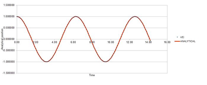
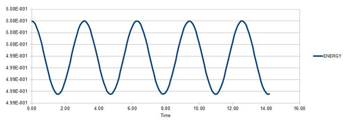
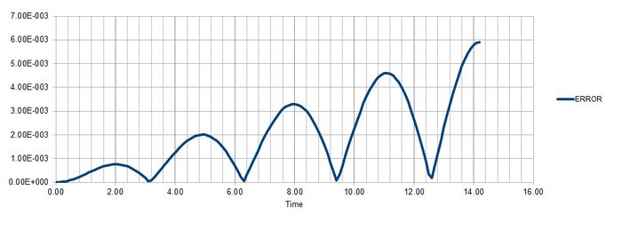
Maximum error is found at Time = 2, 4.9, 8, 11.1, 14.2 for timestep 0.1.

Figure 4: Showing the positions of maximum error, fitted with a trend line and function

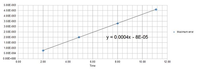
Figure 4 shows the function of the maximum error as $y=0.0004x-8\times 10^{-5}$ where y = error and x = time.

JC: Why does the error oscillate?

Task 3

The timestep must be less than or equal to 0.2 in order to avoid a change in error greater than 0.005, which is a 1% change. If the energy increases largely, it is an indication that the simulation is incorrect because the total energy of a system experimentally will always want to decrease.

JC: Energy doesn't always decrease, total energy should be conserved.

Task 4

Finding the separation, $r_0$, at which the potential energy is 0:

$\varphi \left(r\right)=4ϵ(\frac{{\sigma }^{12}}{r_0^{12}}-\frac{{\sigma }^6}{r_0^6})=0$

Assumed that:

$(\frac{{\sigma }^{12}}{r_0^{12}}-\frac{{\sigma }^6}{r_0^6})=0$

If $r_0=\sigma$ then $(\frac{{\sigma }^{12}}{r_0^{12}}-\frac{{\sigma }^6}{r_0^6})=(1-1)=0$

Therefore $r_0=\sigma$

Next the force was calculated at this separation:

$F=\frac{dv}{dr}=4ϵ(-12\frac{{\sigma }^{12}}{r_0^{13}}+6\frac{{\sigma }^6}{r_0^7})$. Substitute $r_0=\sigma$ to obtain $F=4ϵ-6\sigma$.

JC: This is not correct, the force at should be (24*epsilon)/sigma.

Subsequently the equilibrium separation, $r_{eq}$ was calculated:

At equilibrium, $F=\frac{dv}{dr}=4ϵ(-12\frac{{\sigma }^{12}}{r_{eq}^{13}}+6\frac{{\sigma }^6}{r_{eq}^7})=0$.

Assumed that:

$(-12\frac{{\sigma }^{12}}{r_{eq}^{13}}+6\frac{{\sigma }^6}{r_{eq}^7})=0$

And so:

$(2\frac{{\sigma }^{12}}{r_{eq}^{13}}=\frac{{\sigma }^6}{r_{eq}^7})$ so $(2\frac{{\sigma }^{12}}{{\sigma }^6}=\frac{r_{eq}^{13}}{r_{eq}^7})$ so $2{\sigma }^6=r^6$

Substitute back into:

$\varphi \left(r\right)=4ϵ(\frac{{\sigma }^{12}}{r_{eq}^{12}}-\frac{{\sigma }^6}{r_{eq}^6})$

To give:

$\varphi \left(r\right)=4ϵ(\frac{{\sigma }^{12}}{4{\sigma }^{12}}-\frac{{\sigma }^6}{2{\sigma }^6})=4ϵ(\frac{1}{4}-\frac{1}{2})=-ϵ$

This has shown that $ϵ$ is the well depth.

Evaluating the integrals:

$\int \varphi \left(r\right)\mathrm{d}r=4ϵ(\frac{{\sigma }^6}{7r^7}-\frac{{\sigma }^{12}}{13r^{13}})$

$\sigma =ϵ=1.0$

Between $r=2\sigma$ and $r=\mathrm{\infty }$:

$\underset{2\sigma }{\overset{\mathrm{\infty }}{\int }}\varphi \left(r\right)\mathrm{d}r=-0.0248$

Between $r=2.5\sigma$ and $r=\mathrm{\infty }$:

$\underset{2.5\sigma }{\overset{\mathrm{\infty }}{\int }}\varphi \left(r\right)\mathrm{d}r=-0.00818$

Between $r=3\sigma$ and $r=\mathrm{\infty }$:

$\underset{3\sigma }{\overset{\mathrm{\infty }}{\int }}\varphi \left(r\right)\mathrm{d}r=-0.00329$

JC: Correct.

Task 5

There is 1 mL of water present, which equals 1 g. First, calculate moles:

$Moles=\frac{Mass}{M_r}=\frac{1}{18.0}$

Next, multiply by Avogadro's number to calculate the number of molecules present:

$Numberofmolecules=6.02\times 10^{23}\times \frac{1}{18.0}=3.34\times 10^{22}molecules$

The calculation is reversed to find the volume occupied by 10,000 water molecules:

$\frac{10000}{6.02\times 10^{23}}=1.66\times 10^{-20}moles$

Then to calculate mass:

$Mass=M_r\times Moles=18.0\times 1.66\times 10^{-20}=2.99\times 10^{-19}g=2.99\times 10^{-19}ml$

The simulation clearly models very small volumes.

Task 6

The atom moves to $(0.5,0.5,0.5)+(0.7,0.6,0.2)=(1.2,1.1,0.7)$. Taking into account the Periodic Boundary Conditions, this becomes $(0.2,0.1,0.7)$.

Task 7

Calculating the LJ cutoff in real units: $r^{*}=\frac{r}{\sigma }$

$r^{*}=3.2=\frac{r}{0.34}$

$r=1.088nm$

Calculating the well depth, $ϵ$:

$\frac{ϵ}{k_B}=120K$

Using the Boltzmann Constant: $8.31\times 10^{-3}kJ{K}^{-1}mo{l}^{-1}$

$ϵ=8.31\times 10^{-3}\times 120=0.997kJmo{l}^{-1}$

Calculating the temperature in real units, where $\frac{ϵ}{k_B}=120$:

$T=\frac{T^{*}ϵ}{k_B}=1.5\times 120=180K$

JC: Correct.

Section 3: Equilibration

Task 1

Generating atoms in random positions will place them in situations in which they wouldn't naturally be found. The simulation is therefore deviating from reality. For example, two atoms could be generated very close to each other, a configuration which has very high energy and will give an imperfect simulation.

JC: Why is this imperfect? It can generate high repulsive forces making the simulation unstable and causing it to crash.

Task 2

Satisfying that the lattice spacing and density match:

$Density=\frac{N}{V}$

Here the volume is the lattice spacing cubed, while the number of atoms equals one in the unit cell.

$Density=\frac{1}{1.07722^3}=0.800$

Now we are considering a face-centred cubic lattice with a lattice point number density of 1.2. There are four atoms per unit cell, therefore:

$1.2=\frac{4}{(sidelength{)}^3}$

So:

$Sidelength=1.49$

Task 3

4000 atoms would be created in the face-centred cubic lattice because each unit cell contains 4 atoms.

JC: Correct.

Task 4

'mass 1 1.0' means set the mass of atom type 1 to 1.0 in reduced units.

'pair_style lj/cut 3.0' sets the interactions between pairs of atoms. lj/cut means set Lennard-Jones interactions for atoms beyond a distance of 3.0 to 0. This function does not compute a Coulombic interaction.

'pair_coeff * * 1.0 1.0' This is setting the coefficients in the Lennard-Jones potential equation. The asterisks mean apply the following coefficients to all atom types. The first 1.0 sets $ϵ=1.0$ and the second 1.0 sets $\sigma =1.0$, both in energy units.

JC: Correct.

Task 5

We will use the Verlet algorithm.

Task 6

Figure 1: Energy against time for the timestep 0.001

Figure 2: Temperature against time for the timestep 0.001

Figure 3: Pressure against time for the timestep 0.001

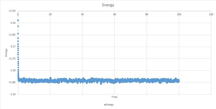
The system reaches equilibrium, within the boundaries $t=0.3$ and $t=0.4$.

Figure 4: Energy vs time for all timesteps. Key: 0.0075 = Blue, 0.0025 = Green, 0.015 = Orange, 0.01 = Yellow, 0.001 = Grey

The best timesteps appear to be 0.001 and 0.0025 because they converge. The larger of these two is 0.0025 so this is the best timestep to use.

Timestep of 0.015 gave particularly bad results. It bears no resemblance to other data and it does not equilibrate.

JC: Good choice of timestep, total energy should be independent of the choice of timestep.

Part 4: Running Simulations under Specific Conditions

Task 1

Determining $\gamma$.

We are given:

$\frac{1}{2}\sum _i{m}_i{v}_i^2=\frac{3}{2}N{k}_{B}T$

Substitute ${\gamma }_i{v}_i$ for $v_i$ and then substitute $\mathfrak{𝔗}$ for $T$ to give:

$\frac{1}{2}\sum _i{m}_i({\gamma }_i{v}_i{)}^2=\frac{3}{2}N{k}_B\mathfrak{𝔗}$

Solve these two equation simultaneously to give:

${\gamma }^2=\frac{\mathfrak{𝔗}}{T}$ and therefore:

$\gamma =\sqrt{\frac{\mathfrak{𝔗}}{T}}$

JC: Correct.

Task 2

It is easier to explain the numbers in reverse order. The third number dictates how often (in terms of timesteps) to take an average. The second number controls how many input values will be used in the average. The first number controls how far apart the input values will be in the average. In this particular simulation, the average is taken every 100,000 timesteps and 1,000 values contribute to each average, with the input values being found 100 timesteps apart.

This simulation will run for 100,000 timesteps.

JC: Good explanation.

Task 3

Figure 1: Density as a function of temperature at $p=2.5$ and $p=3.5$.

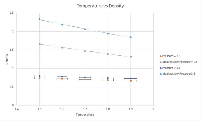
The simulated density is lower. This is because the Ideal Gas Law does not take into account interactions between atoms. Therefore they can get much closer to each other at the same pressure, increasing the density. The simulation considers interactions (as it uses the Lennard-Jones potential), preventing atoms from becoming so close because the potential energy is too high. The discrepancy increases with pressure.

JC: Why do you use a straight line for the ideal gas law, the equation shows that density is proportional to 1/T, not to T. How does the discrepancy change with temperature?

Part 5: Calculating Heat Capacities using Statistical Physics

Task 1

Figure 1: $C_V/V$ as a function of $T$.

This trend is not expected. Heat capacity normally increases with temperature because the degrees of freedom increase. The simulated trend can be explained by the band gap in the crystal getting smaller as temperature increases. Therefore for a given temperature increase, the amount of energy required to promote to the next translational energy level is smaller, hence heat capacity is smaller.

Here is an input file for the NVT ensemble at p=0.2 and T=2.0:

The heat capacity is larger for a larger density. This is because

File:JK2105Nvt0.2,2.0modified.txt

JC: Good attempt at explaining the trend in heat capacity with temperature, more analysis outside the scope of this experiment would be needed to confirm this.

Part 6: Structural properties and the radial distribution function

Task 1

Figure 1: Radial Distribution Functions for Solid, Liquid and Gas

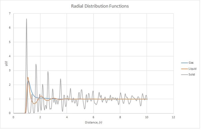
The three different phases show very different distributions. All three show a very low probability until a distance of r=1. This is due to the Lennard-Jones potential being very high. All three phases also show a peak at 1 which is the equilibrium energy, so it is most favourable for neighbours to sit here.

The solid is in a face centred cubic lattice which means that an atom's neighbours are going to be very particular distances away. This explains why there are sudden peaks and troughs in probability.

The liquid is more diffuse and fits a weak, almost lattice-like, pattern while the Lennard Jones potential is favourable. Further away, the distribution becomes random. It is equally likely to find an atom at any distance at high (r).

The gas is very disordered and is distributed completely randomly, though the probability is higher while there is a favourable Lennard Jones potential. The average probability tends to 1 as the Lennard-Jones potential tends to 0.

Figure 2: Diagram showing the three atoms which the first three peaks on the solid RDF diagram correspond to.

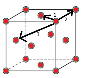
Figure 2 illustrates which are the closest three lattice positions to the central atom. These are therefore the three first peaks in the RDF graph.

The lattice spacing equals 1.375, the x-value of the second peak on the RDF graph, as this is the second closest position to the central atom.

Figure 3: Cumulative integration of Solid RDF, used to calculate the coordination number to each lattice position

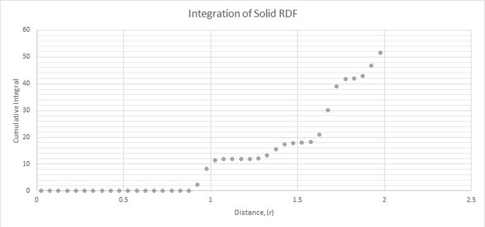
Figure 3 was used to calculate the coordination number for the first three peaks. The central atom coordinates to the closest position (marked 1 in figure 2) 12 times. It coordinates to the second closest position 6 times and to the third closest position 24 times.

JC: The radial distribution function tends to 1 as it is normalised by the bulk density. Good idea to include a diagram of an fcc lattice to show which atoms are responsible for the peaks. Could you have calculated the lattice parameter from the first and third peaks as well and taken an average?

Task 6: Dynamical Properties and the Diffusion Coefficient

Task 1

Using data from simulation

For the following graphs, the series Timestep was replaced by Time, which was achieved by multiplying Timestep series by a tenth of the simulation timestep (0.002).

Figure 1: Mean Squared Displacement of the gas as a function of Time. The gradient of the linear section = 1.41

Figure 2: Mean Squared Displacement of the liquid as a function of Time. The gradient of the line = 0.0509

Figure 3: Mean Squared Displacement of the solid as a function of Time. The gradient of the line is assumed to be zero at equilibrium.

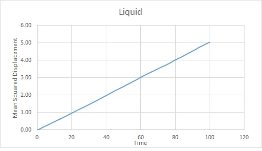
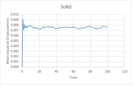
The trends are as expected. The gas becomes the most displaced as it is the most disordered phase. The rate of change of displacement increases until about timestep 2000. This is probably because the gas has diffused sufficiently to overcome Lennard Jones Potential at this point. It will continue to diffuse.

The liquid becomes more diffuse with time but at a much slower rate than the gas because it has stronger interactions between particles.

The solid rapidly takes its lattice position as this is energetically favourable. It will oscillate slightly before remaining in the lattice. Although there is a slight translation, the scale shows that this is very small so the position varies very little from its average.

Estimation of $D$, the Diffusion Coefficient:

$D=\frac{1}{6}\frac{\partial ⟨r^2\left(t\right)⟩}{\partial t}$

Using the gradients of the linear sections of the graphs, as mentioned above:

Gas: $D=\frac{1}{6}\times 1.41=0.235$ Reduced units

Liquid: $D=\frac{1}{6}\times 0.0509=0.00848$ Reduced units

Solid: $D=\frac{1}{6}\times 0=0$ Reduced units

Data from one million atom simulations

Time could not be calculated as the simulation's timestep was not given:

Figure 4: Mean Squared Displacement of the gas as a function of Timestep. The gradient of the linear section = 0.0376

Figure 5: Mean Squared Displacement of the liquid as a function of Timestep. The gradient of the linear section = 0.00105

Figure 6: Mean Squared Displacement of the solid as a function of Timestep. The gradient of the line is assumed to be zero at equilibrium.

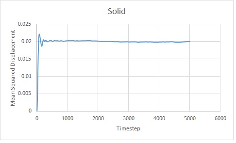
Using the gradients of the linear sections of the graphs, as mentioned above:

Gas: $D=\frac{1}{6}\times 0.0376=0.00627$ Unknown units

Liquid: $D=\frac{1}{6}\times 0.00105=0.000175$ Unknown units

Solid: $D=\frac{1}{6}\times 0=0$ Unknown units

JC: Show the linear fits on the graphs.

Task 2

Evaluating the normalised velocity autocorrelation function for a 1D harmonic oscillator:

Figure 7: VACF evaluation

Figure 8: VACF evaluation part 2

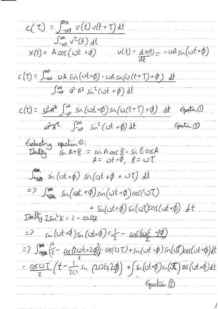
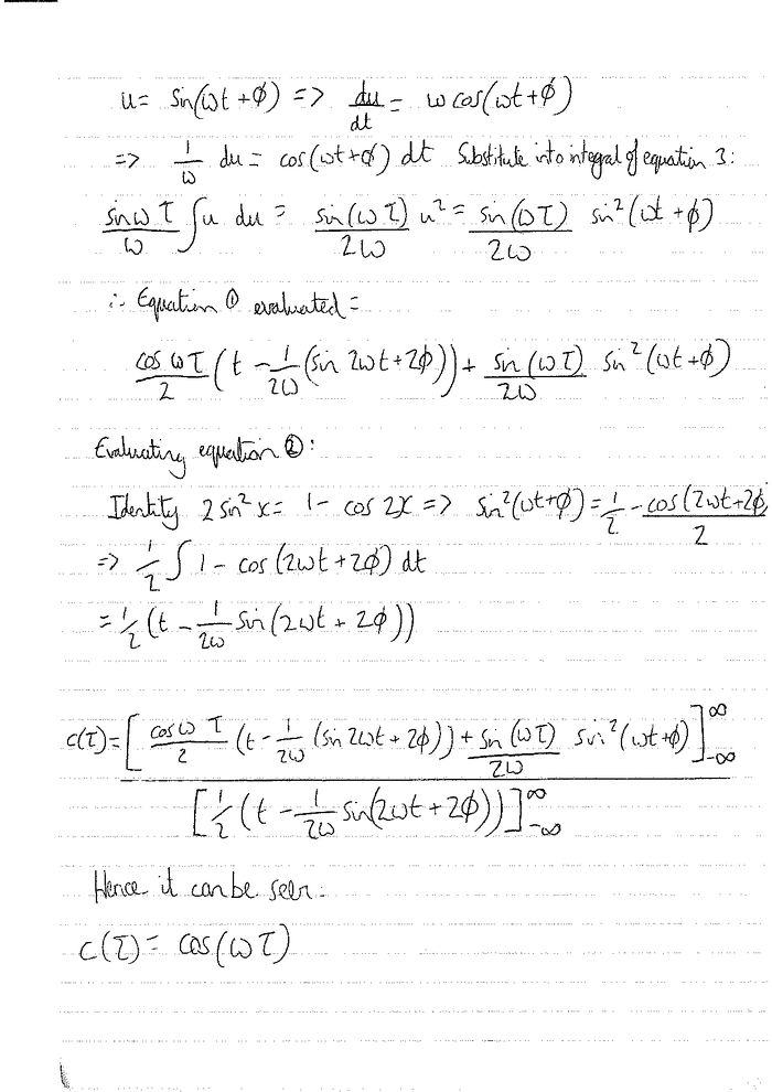
JC: Rather than actually performing the integration, the integral in the numerator can be simplified into a sin squared term which cancels with the denominator and a sin x cos term which is zero since it is an odd function.

Figure 9: The VACF for a harmonic oscillator, solid and liquid plotted for timesteps 0 to 500.

JC: Can you explain the shape of the VACF and the differences between the harmonic oscillator and simulation data?

Task 3

The trapezium rule was used to evaluate the area beneath the graphs for my own simulation. This gave an integration of -5.39 for the solid, -5.39 for the liquid and 3499 for the gas. The diffusion coefficient, $D$ was calculated in each case: $D_{solid}=\frac{1}{3}\times -5.39=-1.80$

$D_{liquid}=\frac{1}{3}\times -5.39=-1.80$

$D_{gas}=\frac{1}{3}\times 3499=1166$

Figure 9: Running integration using the trapezium rule for solid and liquid. The two integrations overlap.

JC: This doesn't look like the running integral for the solid or liquid, is this actually for the harmonic oscillator?

Figure 10: Running integration using the trapezium rule for gas.