Talk:Mod:JAS213

Year 3 Computational Experiment - Liquid Simulations

Velocity Verlet Algorithm

Task 1

Analytical:

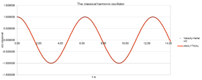
The Analytical solution is the position calculated with the classical approach using the harmonic oscillator. It was obtained by plugging the given values for A,$\omega ,\varphi$ into the following 1D harmonic oscillator position function: $x(t)=A\cos (\omega t+\varphi )$ $A=1.0,\omega =1.0,\varphi =0$

The values obtained from the analytical harmonic oscillator and the Velocity-Verlet algorithm match up nicely, because the analytical joins up the points of the velocity-Verlet solution.Thus, the classic harmonic oscillator solutions and the ones obtained by the velocity-Verlet solution are in good agreement. The difference between these two solutions is obtained by calculating the ERROR. See below “Error” section.

Fig. 1. The classic harmonic oscillator and the velocity-verlet solution vs. time

Energy:

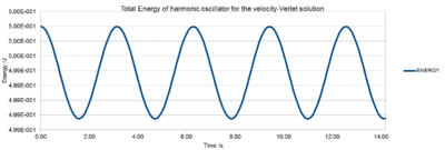
The total Energy of the harmonic oscillator is calculated by the sum of the potential and the kinetic Energy:

$E_{TOTAL}=\frac{1}{2}k{x}^2+\frac{1}{2}m{v}^2$

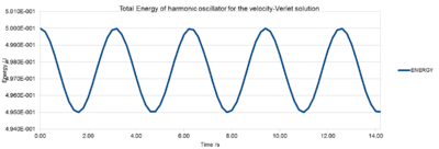
For an isolated system such as our simulation box, no exchange should happen between system and surroundings and we would expect the total energy to be constant. The Energy is however not completely constant, since in a harmonic oscillator a periodical motion of compression and expansion occurs alternatively. Nonetheless, these fluctuations are so small, that the overall total energy can be considered as constant. Generally speaking, throughout all simulations, the total energy should be monitored to ensure good results and an isolated system.

NJ: No! The analytical solution conserves energy exactly. The fluctuations that you see are a consequence of the Verlet algorithm.

Fig.2 Total Energy of harmonic oscillator for the velocity-Verlet solution

Error:

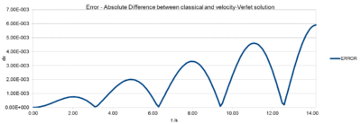
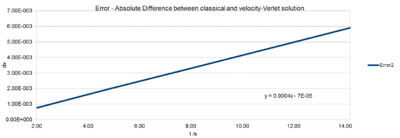
The error is the absolute difference between the velocity-Verlet position and the Analytical harmonic oscillator position calculated above (Fig.1). To obtain solely positive values, "=ABS(C6-F6)" the absolute was used in Excel. Note: The absolute difference in positions between classic harmonic oscillator and the velocity-Verlet solution increases with time. This is due to the fact, that the velocity-Verlet solution builds up the error from the previous calculations. The error varies periodically, but , but the amplitude of the peaks, hence the maxima increase over time. The gradient for this linear increase in amplitude can be read off Fig. 4 The Error maxima vs. time plot and is $4x10^{-4}$.

Fig. 3 The error vs. Time plot

Task 2:

The positions of maximum error have been estimated for the default value 0.1 as a function of time. It can clearly be seen that the error increases linearly with time. The error is build up in the verlet algorithm. (Section 2.3 http://physics.bu.edu/~py502/lectures3/cmotion.pdf)

Fig.4 The Error maxima vs. time plot

Task 3:

A timestep of 0.20 is needed to ensure that the total energy of the harmonic oscillator does not change by more than 1 % over the course of the simulation. In case of 0.20, the total energy varies between 0.5 (the initial value) and 0.495.

This simulation relies on the harmonic oscillator whose overall total energy should be constant. However, due to its non-chaoticonic oscillating system we observe periodic variations. For your simulations you would want the system to have a constant energy throughout. Therefore, it is extremely important to monitor these energy fluctuations. A good simulation should have a time independent constant total Energy. Because of the harmonic oscillator, the initial value is the one closest to reality (0.50). Thus, the total energy maxima on Fig. 2. represent the correct values, whereas the minima (0.495 for 0.2 timestep) represent the largest deviation from reality. As long as we are aware of these changes, these small periodic fluctuations do not cause any problems, since the overall total energy remains constant. An unacceptable simulation would be one, where the total Energy would increase or decrease over time.

NJ: Good

Fig.4 Total Energy of harmonic oscillator for the velocity-Verlet solution for a steptime of 0.2

Atomic Forces

Task 1

a)Calculation of the position of zero potential r₀:

$\varphi (r)=4ϵ(\frac{{\sigma }^{12}}{r^{12}}-\frac{{\sigma }^6}{r^6})$ (1)

Since $r_0$ is the position at which $\varphi (r)=0$, (1) simplifies to:

$\frac{{\sigma }^{12}}{r^{12}}-\frac{{\sigma }^6}{r^6}=0$

4ε is a constant, thus $r_0=\sigma$. (2)

b) Force at r₀:

The Force at $r_0$ is given by the first derivative $F_0=\frac{d\varphi (r)}{d{r}_0}$

$\sigma$ is plugged into the equation, instead of $r_0$, since (2).

$\frac{d\varphi (r)}{d{r}_0}=4ϵ(\frac{-12{\sigma }^{12}}{{r_0}^{13}}+\frac{6{\sigma }^6}{r_0^7})$

$=4ϵ(\frac{-12}{\sigma }+\frac{6}{\sigma })$

$=4ϵ(\frac{6}{\sigma })$

$=\frac{24ϵ}{\sigma }$

c) Determination of the equilibrium separation r_eq and the well depth ε

From the Lennard-Jones potential, we know that the equilibrium bond length is found at the minimum Lennard-Jones interaction. Thus, the first derivative of $\frac{d\varphi (r)}{dr}$ must be equal to zero:

For$r=\sigma$

$\frac{d\varphi (r)}{dr}=4ϵ(-12+\frac{6}{\sigma })$

$\frac{48ϵ{\sigma }^{12}}{r^{13}}=\frac{24ϵ{\sigma }^6}{r^7}$

$\frac{48ϵ{\sigma }^{12}}{24ϵ{\sigma }^6}=r^6$

$2{\sigma }^6=r^6$

$\sqrt[6]{2}\sigma =r_{eq}$

The well depth $\varphi r_{eq}$:

$\varphi (r_{eq})=4ϵ(\frac{{\sigma }^{12}}{r^{12}}-\frac{{\sigma }^6}{r^6})$

If we plug the previously obtained relationship ($r_{eq}=\sqrt[6]{2}\sigma$) into $\varphi (r_{eq})$ we obtain the well depth ε at the equilibrium position:

$\varphi (r_{eq})=4ϵ(\frac{{\sigma }^{12}}{4{\sigma }^{12}}-\frac{{\sigma }^6}{2{\sigma }^6})$

$=4ϵ(\frac{1}{4}-\frac{1}{2})$

$=\frac{-4}{4}ϵ=-ϵ$

The equilibrium potential is equal to the negative well depth.

d) Integral Evaluation when σ=ε=1.0

$\underset{2\sigma }{\overset{\mathrm{\infty }}{\int }}4ϵ(\frac{{\sigma }^{12}}{r^{12}}-\frac{{\sigma }^6}{r^6})dr$

$=4[\frac{-r^{11}}{11}+\frac{r^{-5}}{5}{]}_2^{\mathrm{\infty }}$

$=0-4(\frac{-2^{11}}{11}+\frac{2^{-5}}{5})$

$=-\frac{699}{28160}$

$=-2.48x10^{-2}$

$\underset{2.5\sigma }{\overset{\mathrm{\infty }}{\int }}4ϵ(\frac{{\sigma }^{12}}{r^{12}}-\frac{{\sigma }^6}{r^6})dr$

$=4[\frac{-r^{11}}{11}+\frac{r^{-5}}{5}{]}_{2.5}^{\mathrm{\infty }}$

$=0-4(\frac{-2.5^{11}}{11}+\frac{2.5^{-5}}{5})$

$=-8.18x10^{-3}$

$\underset{3\sigma }{\overset{\mathrm{\infty }}{\int }}4ϵ(\frac{{\sigma }^{12}}{r^{12}}-\frac{{\sigma }^6}{r^6})dr$

$=4[\frac{-r^{11}}{11}+\frac{r^{-5}}{5}{]}_3^{\mathrm{\infty }}$

$=0-4(\frac{-3^{11}}{11}+\frac{3^{-5}}{5})$

$=-3.29x10^{-3}$

The integral becomes rather small, as the near distance is increased.This near distance represents the cutoff distance, which becomes less significant as increased, since the atomic interactions decrease with distance.

NJ: Nicely presented

Periodic Boundary Conditions

Task 1

When calculating the number of water molecules contained in 1 mL of water, we can use the famous relationship that 1 L of water contains 55 mol Water molecules, which was obtained as follows:

$\frac{1000mL}{1L}\frac{1g}{1mL}\frac{1mol}{18g}=55.56mol{L}^{-1}$

Thus, for the exact number of water molecules in a volume of 1 mL, we multiply the result above by Avogadro's Number N_a and divide by 1000:

$\frac{55.56mol}{1L}=\frac{55.56x6.022x10^{23}}{1000mL}=3.35x10^{22}$ water molecules per 1 mL

Task 2

Now, looking for the Volume: $V=\frac{m}{d}$

Pluggin into $n=\frac{m}{M}$

$V=\frac{n*M}{d}$

$=\frac{\frac{10000}{6.022x10^{23}}*18g}{1gc{m}^{-3}}$

$=2.99x10^{-19}c{m}^3$

Task 3

The initial position is(0.5, 0.5, 0.5), the box runs from (0,0,0) to (1,1,1). After timestep, when it moves along the vector(0.7, 0.6, 0.2). The new position is going to be (0.2,0.1,0.7).Our box size is 1 in each direction and so due to the periodic boundary conditions: If anything leaves the box, it will come in on the other side. This case applies for x and y in the above example.

Task 4

All simulations use reduced units, thus graphs are all given in reduced units and it is important that we can convert back into real units. For Argon, the real units are:

Distance

$r=r*\sigma$

$=3.2*0.34$

$=1.088nm$

Well depth

$ϵ=120K*K_B$

$=120K*1.38*10^{-23}*10^{-3}kJ{K}^{-1}*6.022*10^{-23}mo{l}^{-1}$

$=0.997kJmo{l}^{-1}$

Temperature

$T=\frac{ϵT^{*}}{k_B}$

$=\frac{120K*k_B*1.5}{k_B}$

$=180K$

Equilibration

Task 1

TASK: Why do you think giving atoms random starting coordinates causes problems in simulations? Hint: what happens if two atoms happen to be generated close together?

Giving atoms random starting coordinates for the simulations causes problems, because the atoms could end up very close to each other or even overlapping each other. If two atoms are generated very close together, they feel a very high repulsive force, corresponding to the $-r^{-12}$term of the Lennard-Jones potential. Thus, the atoms want to move away from each other as quickly as possible. This results in an increase in velocity. These "high-speed" atoms may bump into other atoms while moving away from each other, increasing the overall chaotic kinetic energy, T, resulting in an increase in temperature and thus in an increase of the total energy of the system. This behaviour is characteristic for explosion.

NJ: Up to this point the explanation is very good.

Therefore, for a dense system, the atoms are usually placed at the vertices of a face-centered cubic lattice, which tends to minimize the potential energy."_[1]

NJ: Not necessarily, it depends on what you're simulating.

The actual problem for our simulation is that the system is only simulated for a short period of time and this is why the starting position should be close to equilibrium to get good results._[1]

In case of the atoms being very close together, the chosen timestep might be too big to monitor the movement of the very quick accelerated movement of the atoms. Therefore a very small timestep would be necessary.

NJ: Yes, good.

Task 2

Face Centered Cubic Lattice

Simple Cubic Lattice

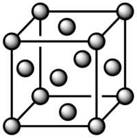
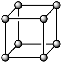
The number density of lattice points for a simple cubic lattice is 0.8. This value was obtained using the following: N= The number of lattice points $N=\frac{4}{4}=1$

r^*= Distance between the lattice points in reduced units

$\rho =\frac{N}{V}$

$=\frac{1}{1.07722^3}$

$=0.79999$

$=0.8$

For a face centered lattice with a number density of lattice point of 1.2: $N=\frac{4}{4}*\frac{6}{2}=4$

$r^{*}=\sqrt[3]{\frac{4}{1.2}}=1.49$

Task 3

For a face centered cubic lattice, the number of lattice points and atoms coincide. Thus, one unit cell has 4 atoms and we are looking at a box with 1000 unit cells. The total number of atoms is: $4*1000=4000$

Task 4

From the LAMMPS manual:

LAMMPS command "mass 1 1.0"

The command "mass" means that it sets the mass for all atoms of one or more atom types. The value "1" in the middle is the Index value and specifies the mass for only one atom type is set. This makes sense, since our previously defined box contains only one atom type. The value on the right "1.0" is the actual value to which the mass is set.

LAMMPS command "pair_style lj/cut 3.0"

This command sets the formula(e) LAMMPS uses to compute the pairwise interaction. Pair potentials are in LAMMPS defined between atom pairs, that are within the cutoff distance. The set of active interactions typically changes over time. "lj" is the style and "cut" is the argument used. This specific lj command means that the Lennard-Jones potential with no Coulombic interactions is used. The "cut" part indicates that the cutoff distance is at 3.0. This command seems reasonable, since we know from the calculation of the integral, that the interaction becomes insignificantly small with increasing the nearer limit $2\sigma$ to $3\sigma$.

LAMMPS command "pair_coeff * * 1.0 1.0"

This command specifies the pairwise force field coefficients for one or more pairs of atom types. The general syntax of this command is "pair_coeff I J args" where I,J indicate the atom types (see asterisk form below), args stands for the coefficients of one or more pairs of atom types. A wildcard asterisk can be used instead of or in combination with the I,J arguments to set the coefficients for multiple pairs of atom types. In this example the coefficients of all atom types from 1 to N are set to 1.0. If the left asterisk was as number eg. 3, the command would only include all types from 3 to N (inclusive). If the right asterisk was replaced with 3 and the left kept, the command would only include all types from 1 to 3 (inclusive). In this case with two asterisks and no numbers, all atom types from 1 to N (inclusive) are included and set to 1.0. Because we are dealing with a symmertric J,I interaction, the coefficients following J,I are set to the same values: Thus the force field coefficients are the same resulting in a symmetric interaction. This means that the lennard jones potential is at equilibrium distance. Then, the coefficients can be related to the well depth ε ie. measures how strongly two particles attract each other and σ ie. the distance at which the intermolecular potential between two particles is zero. For the exact relationship between these two quantities, refer to [3]. To put it in a nutshell, the pairwise force field coefficients measures how close two non bonding particles can get together and is therefore also known as the van der Waals radius.

[3]http://www.csb.yale.edu/userguides/datamanip/autodock/html/Using_AutoDock_305.a.html#29613

Task 5

Given that the initial position x_i(0) and the initial velocity v_i(0) are necessary for the integration, the velocity-Verlet algorithm is used. The classic Verlet algorithm, another numerical integration method, would not require the initial velocity.

Task 6

Comparing the two LAMMPS commands given in the script:

In the simple example, the timestep is set to a constant value, and then a "run" command is used. This simply means that the dynamics simulation is run or continued until it reaches 100000 timesteps. This simple 2 line command focusses only on one property, the timestep and applying it for a certain number of times. It would be a usable command, if the timestep was never changed. This is however not the case.

Therefore, the first longer command is used, because it incorporates the floor() function from the C math library. The floor is used to maintain the same duration for each simulation, no matter what timestep is chosen. The floor function is the right choice because the largest integer (obtained from the division) will not be greater than its argument (100 000). To sum up, it ensures that the number of steps is multiplied by a certain time dt. In this waz, each simulation runs for the same amount of time, no matter what timestep has been chosen.

NJ: Good

Fig.5 Reduced Energy vs. time.png

Fig.5 Reduced Temperature vs. time.png

Fig.5 Reduced Pressure vs. time.png

Task 7

For a timestep of 0.001, it can be seen from the reduced total Energy vs. time, the reduced pressure vs. t and the reduced Temperature vs. t plot, that equilibrium is reached at approximately 0.35 s. This number was obtained by zooming in on Fig.5 Reduced Energy vs. Time. However, pressure and temperature of the system also reach a constant average value, as well with fluctuations obviously.

Fig.6 Reduced energy vs. time different timesteps.png

The largest timestep to give acceptable results is 0.010 (yellow), because it is the largest to display constant energy.

NJ: Yes, but the average energy that you get also seems to depend on the timestep - as you make the timestep smaller, the average energy decreases (up to a point). 0.0025 is the best timestep, because that is the point at which the average energy seems to have converged (i.e. when the timestep is made even smaller, 0.001, the value of the energy isn't affected).

A particularly bad choice of timestep would be 0.015 (top blue), because at this stepsize we have decreased the degree of accuarcy of our result, since the Energy is not constant anymore. It is decreasing with time. Additionally, the fluctuations seem to have increased a lot, resulting in an increase in the standard derivation.

Running simulations under specific conditions

Temperature and Pressure Control

NpT (isobaric-isothermal) ensemble, from the previous section the largest timestep, which still shows constant energy, pressure and temperature of 0.01 was used. By taking the average from each of the five Intro simulations, the average pressure of 2.60 was obtained.

A pressure of 2.6 and 3.0 was used with Temperatures varying from 1.6, 2.0, 2.4, 2.8, 3.2

Thermostats and Barostats

We need to choose $\gamma$ so that the temperature is correct $T=\mathfrak{𝔗}$ if we multiply every velocity $\gamma$. We can write two equations:

$\frac{1}{2}\sum _i{m}_i{v}_i^2=\frac{3}{2}N{k}_{B}T$ (1)

$\frac{1}{2}\sum _i{m}_i{\left(\gamma v_i\right)}^2=\frac{3}{2}N{k}_B\mathfrak{𝔗}$ (2)

From the first equation, we know that the left hand side (LHS) of (2) without the $\gamma$ is equal to the right hand side (RHS) of (1). Therefore:

$\frac{3}{2}N{k}_{B}T{\gamma }^2=\frac{3}{2}N{k}_B\mathfrak{𝔗}$

$T{\gamma }^2=\mathfrak{𝔗}$

${\gamma }^2=\frac{\mathfrak{𝔗}}{T}$

$\gamma =\sqrt{\frac{\mathfrak{𝔗}}{T}}$

Now, if $T=\mathfrak{𝔗}$,

$\gamma =1$

Examining the Input Script

### MEASURE SYSTEM STATE ###
thermo_style custom step etotal temp press density
variable dens equal density
variable dens2 equal density*density
variable temp equal temp
variable temp2 equal temp*temp
variable press equal press
variable press2 equal press*press
fix aves all ave/time 100 1000 100000 v_dens v_temp v_press v_dens2 v_temp2 v_press2
run 100000

By examining the second last line "fix aves...", we note that 100=Nevery 1000=Nrepeat and 100000=Nfreq. Therefore, values on timesteps 100 200 300 400 500 600... until 100000 will be used to compute the final average on timestep 100000. Nfreq determines on how often the average is calculated. In this example it is calculated every 10000 timesteps. Nfreq must be a multiple of Nevery and Nevery must be non-zero even if Nrepeat is 1. N every just tells us which input values are going to be used as samples for the ave/time measurements. N repeat tells us how many measurements of this repeated Nevery number of timesteps apart are going to be used.

The last line tells me that the simulation is run for 100000 timesteps. My previously set timestep is 0.01 (the largest that still gives reasonable resutls). Even better would be the smaller timestep of 0.0025, which is used in the following input files, giving a reduced time of 250. From the LAMMPS manual examples I infer that the units are fmsec. So the simulation is running for 0.01*100000=1000 fms, femtoseconds or with the smaller timestep for 250 fms.

NJ: The units are dimensionless. So it's 1000 time units, not 1000 femtoseconds.

Plotting the Equations of State

Fig. 9 Number density vs. Reduced Temperature

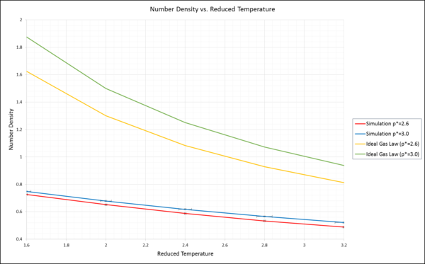
NJ: Nice plot, but don't just use lines to "join up" points. You can either generate more data points for the ideal gas curve (which you know is continuous), so that the line is smoother, fit a function to the data points and plot that, or just plot the points without a line.

Error bars in the x and y direction have been added. However, due to the inclusion of the ideal gas plots, these are now hard to see. Please refer to previous version of this document to double check. There is an observable increase in standard error for the reduced temperature as the same is increased.

The number density${\rho }_N$ expressed by the ideal gas law:

$pV=nRT$

$\frac{p}{k_{B}T}=\frac{n{N}_A}{V}$

$\frac{p}{k_{B}T}=\frac{N}{V}$

$\frac{p}{k_{B}T}={\rho }_N$

However, we are working with reduced units only. Thus, k_B=1.

$\frac{p}{T}={\rho }_N$

General observation:

The simulated Number density is much lower than the Number Density obtained from the ideal gas equation. This discrepancy is coherent with the two models. Due to the fact that the ideal gas law neglects any intermolecular interactions, the number density obtained is higher than the real and the simulated one. The simulated Number Density is much closer to reality, as it is based on Statistical Thermodynamics, which takes intermolecular interactions into account. In the Introduction, we have learned that in this simulation the Lennard Jones potential is the key equation used. The Lennard Jones potential takes intermolecular interactions into account by differentiating between a repulsive $r^{-12}$ an attractive term $r^{-6}$ and is closer to reality.

NJ: Yes, it's wrong because the LJ fluid isn't anything like an ideal gas under these conditions. Can you say more about why the density is lower in the simulated system?

Discrepancy with respect to Pressure:

This discrepancy increases as the pressure increases. For example for the first data point, the discrepancy for p*=2.6 is Δ=0.899, whereas for p*=3.0 the difference is Δ=1.127. Therefore, the higher the pressure, the higher the discrepancy between ideal number density and the simulated one. This seems reasonable, as in the ideal case, we neglect any intermolecular interactions. However, when increasing the pressure, these intermolecular interactions increase. The ideal gas solution does not take them into account, the simulation however does. Therefore the discrepancy increases with increasing pressure.

NJ: Good

Discrepancy with respect to Temperature:

Going along the x-axis of reduced temperature, in both examples the discrepancy between the ideal and the simulated graph decreases notably. To explain this behaviour, the temperature has to be understood as the average chaotic kinetic energy. The Lennard Jones potential becomes less important with increasing average kinetic energy, since the overall total energy is the sum of the potential and the kinetic energy. As stated in the general observation, the Lennard Jones potential is the critical factor determing the discrepancy between the two graphs. This term loses its importance with increasing temperature for the simulation. This is why the graphs come closer together as the Temperature is increased.

NJ: Good effort. A more complete way of explaining this would be something like: 'In an ideal gas, there are no interactions between atoms. The system has only kinetic energy. In the simulated system, atoms interact according to the Lennard-Jones potential. The repulsive interactions prevent atoms from approaching each other closely, decreasing the density with respect to the ideal gas. As pressure increases, density also increases; as the density increases, atoms get closer together and the repulsive interactions become stronger. The discrepancy with the ideal gas law thus increases. As temperature increases, the kinetic energy of the atoms also increases, and the atoms become more able to overcome the repulsive interactions between themselves. The system thus becomes more like the ideal gas, and the discrepancy decreases.

Heat Capacity Calculation

Decrease in specific heat capacity for increasing reduced temperature:

V is the volume of the simulation cell for both densities. Thus, the specific heat capacity can be regarded as just divided by a constant. It is the heat capacity per volume.

Fig. 10 Specific heat capacity over volume vs. Reduced Temperature

File:Jasfig input.txt

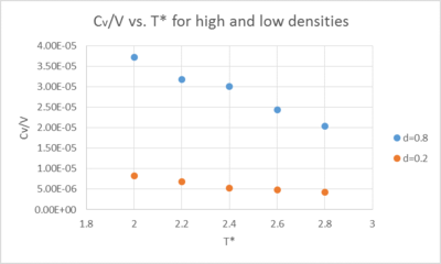
At a high reduced temperature T2 eg. 2.8, the Energy levels are much closer together than at lower Reduced Temperature T1 eg. 2.0. Therefore for the same change in heat dq, at high T* the temperature changes by a larger amount than at low T* where the levels are far apart:

$d{T}_2>d{T}_1$

$C_v=\frac{d{q}_v}{dT}$

Thus, the denominator increases leading to a lowering in Cv/v with increasing T*.

NJ: You can use this argument analogously here, but you have to explain a bit more - this isn't a quantum system, so it doesn't have energy levels per se. We can still talk about there being "modes" though, which do become more closely spaced in energy at higher temperatures.

how does the heat capacity/v vs. T* changes with d?

At higher density, the atoms are closer together, making it easier for the atoms to transmit energy among them. Therefore, the system can take in a lot of energy at a given temperature.

NJ: These two things aren't quite the same though. The same argument does mean that you have more degrees of freedom per volume in which to store heat, though.

The specific heat capacity at const. V (Cv/V) is therefore increasing with increasing density. When the atoms are further apart, the chaotic kinetic energy is transmitted less easily among the system, lowering its ability to take in heat.

NJ: There's no such thing as chaotic kinetic energy, it's just kinetic energy. Heat capacity (*not* specific heat capacity, that is C/mass, and isn't what you've worked out) is extensive.

Radial Distribution Function

Conditions used for the simulations:

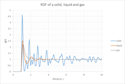
solid: T=1.2 Density=1.2

liquid T=1.2 Density=0.8

gas T=1.2 Density=0.07

Fig. 11 RDF vs. r for solid, liquid and gas

The Lattice spacing:

In the solid case, the lattice spacing can be obtained by looking at the log output file from the lammps calculation. It states the following:

Lattice spacing x,y,z = 1.4938 1.4938 1.4938

NJ: That just tells you the lattice spacing you started with. Only the RDF can tell you what the average spacing actually was over the course of your simulation.

Fig. 12 FCC Unit cell

Calculating r₁ for peak 1:

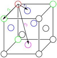
By looking at the first peak in the VMD graph (Fig. 11), from the x value we know: r1= 1.025

Calculated using the LAMMPS log file: $r_1=\sqrt{(\frac{x}{2}{)}^2+(\frac{y}{2}{)}^2}$

$r_1=\sqrt{(\frac{1.4938}{2}{)}^2+(\frac{1.4938}{2}{)}^2}$

$r_1=1.0$

rounded to one decimal place.

Calculating r₂ for peak 2:

From the sketch of the fcc lattice: the distance r between the reference atom and the green atoms is given by x,y or z. Therefore no calculation needs to be done, the result is 1.5 and this corresponds to peak 2 at 1.475.

Fig. 13 Number of Atoms vs. distance Peak 1-3

Fig. 14 Number of Atoms vs. distance

Calculating r₃ for peak 3

By looking at the VMD graph, the peak is at (1.825/2.6) Thus :$r_3$ should be around 1.825:

$r_3=\sqrt{{r_1}^2+z^2}$

$r_3=\sqrt{(1.0{)}^2+(1.4938{)}^2}$

$r_3=1.8$

NJ: You've slightly got the wrong end of the stick here, but your maths is good. I wanted you to estimate the lattice spacing using your RDF, rather than reading it from the log file and then approximating where the peaks should occur. You would then have obtained three estimates for a, the lattice spacing, which you could have averaged.

Discuss qualitatively the differences between the three RDFs and what this tells you about the structure of the system in each phase

The RDF is looking at the numbers of nearest neighbours around one reference atom inside the structure.

NJ: It is the probability of finding a neighbour at a distance, rather than the number of neighbours, and it is averaged over all atoms in the structure.

For the gas (grey), we observe only 1 peak, indicating one first set of nearest neighbours, and no other noticable order in the system. However, for the liquid we can at least spot three noticable peaks, with decreasing amplitude, indicating the presence of the first set of nearest neighbours, the 2nd NN and third NN (without zooming in, orange line)and some sort of order of the system. For the solid there are many more peaks, indicating a highly ordered system. Especially, the first peak is extremely big. At this peak, the density p(r) for several touching neighbours is much bigger than for the bulk density. Thus, g(r)>>1. Peaks are observed throughout, obviously with decreasing intensity. Nonetheless, this clear trend proves the existence of a lattice structure and therefore the above calculations could be performed. The fact that it is a face centered cubic lattice, allows us to assign the exact peaks in the question below.

NJ: We generally characterise the phases as follows: gas, no order; liquid, short range but no long range order; crystalline solid, long and short range order.

The minima between the peaks indicate a space between two sets of nearest neighbours with fewer atoms and thus g(r)<0.

On the far left of the plot, it is in every case equal to zero, until it roughly reaches a distance of r=1. This initial bit of the graph, where g(r)=0 is the region of zero probability of finding an adjacent atom.

NJ: Why do you think this is?

When looking at the right of the graph, g(r) tends towards1 for a large distance r. Therefore, as we move away from the reference atom, the interaction between the reference atom and its surroundings becomes less significant and the density here equals the bulk density.[4]

In the solid case, what is the coordination number for each of the first three peaks?

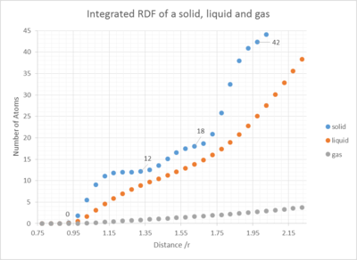
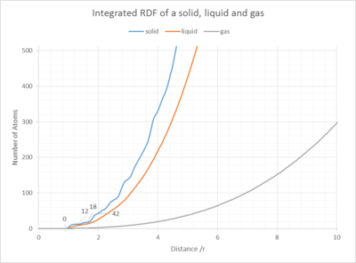
By looking at the different plateaus for the solid integrated RDF G(r) vs. r graph, one can calculate the coordination number to the first nearest neighbours, the second and the third. The coordination number for each peak, each set of nearest neighbours, can be obtained by subtracting the last number on each "plateau", by the last value of the previous "plateau" (See Fig. 12). Using this method, peak 1, the coordination number to the first nearest neighbours (1NN) is 11.8-0.0=11.8, equals 12 atoms. To the second set of nearest neighbours (2NN) it is 18-12=6 atoms (peak 2) and to the third nearest neighbours (3NN) it is 42-18=24 atoms. This results is coherent with the amplitude of the peaks, indicating a high density in close proximity and high amplitude for the 3rd peak, however a smaller for the second due to the fact that peak 1 and peak 3 represent 12 and 24 atoms, whereas peak 2 only represents 6. The theoretical picture agrees with this observation: For =r₁, r₂ and r₃, if we tried to extend the unit cell and imagine the neighbouring unit cells next to our reference atom in 3D space in Fig. 12. We would expect to see 4x3 blue atoms, thus 12 blue; 3x2 green and 6 green atoms.

NJ: Good

Dynamical properties and the diffusion coefficient

Fig.15 Solid MSD vs. timestep

Fig.16 liquid MSD vs. timestep

Fig.17 Gas MSD vs. timestep

Task 1

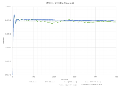
Fig. 15 shows the mean square displacement plotted against timestep for a solid. The MSD seems to increase at the start of the experiment, this is however only due to the fact that we observe ballisitic movement at the start rather than a displacement. NJ: Rather than Brownian motion, but well spotted. The relationship we are interested in, can be seen after 200 timesteps. The mean squared displacement then remains constant. This is due to their fixed position in the face centered cubic lattice.The minor fluctuations are due to the fact, that the atoms are still vibrating inside the lattice. Only at 0 K, a completely straight line should be observed. NJ:A completely straight horizontal line.

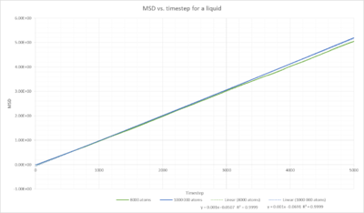
Fig. 16 shows the linear relationship between MSD vs. timestep for a liquid. The mean squared displacement increases linearly with timestep. The completely straight line indicates that only diffusion occurs. Therefore this trend is expected. We only observe Brownian motion. We do not observe some sort of electromagnetic drift that would bend the graph upwards. The particles are not constrained, if they were we would observe a plateau formation.

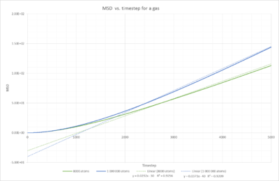
Fig. 17 shows the same linear relationship as the liquid, but with a higher gradient, meaning a higher Diffusivity constant. This is coherent with the states, since particles in a gas should be moving much quicker than particles in a liquid, because in a gas there is a smaller amount of atoms preventing the movement. They are more spread out and therefore the density is lower. Additionally, one should note that the linear relationship cannot be observed right at the start. It takes a certain number of initial timesteps until the simulations reaches this linear relationship, this is due to the initial configuration of the particle within its coordination shell and it takes time until it escapes from it.

NJ: This is again due to ballistic motion

The diffusion constant D is given by the gradient of the MSD:

$D=\frac{1}{6}\frac{\partial ⟨r^2\left(t\right)⟩}{\partial t}$

If we estimate D using the linear trendline y=mx+b:

$D=\frac{1}{6}(\frac{m}{0.002})$

D is the diffusion constant with the S.I. units $m^2{s}^{-1}$ However, the linear equations obtained from the plots are all with respect to timestep and thus unitless (no seconds!). Therefore,all gradients need to be divided by the timestep to obtain D in $m^2{s}^{-1}$. The timestep can be read off the log file and is 0.002 s. Thus, we obtain the following values:

NJ: The timestep is 0.002, not 0.002s!

For the solid:

$D_{3200}=5.8310^{-7}{m}^2{s}^{-1}$

$D_{1M}=4.1710^{-6}{m}^2{s}^{-1}$

For the liquid:

$D_{8000}=8.3310^{-2}{m}^2{s}^{-1}$

$D_{1M}=8.3310^{-2}{m}^2{s}^{-1}$

For the gas:

$D_{8000}=2.43m^2{s}^{-1}$

$D_{1M}=3.10m^2{s}^{-1}$

By comparing the respective D values for the two different numbers of atoms in each state, the values are very similar. For the liquid simulation, no more information is obtained by increasing the number of atoms from 8000 to a million. The correct results are also observed with a smaller number of atoms. The increase in number of atoms to a million makes the calculations more complicate and time consuming, but these result show are smoother and more precise trend.

Task 2

The velocity autocorrelation function:

$C\left(\tau \right)=\frac{\underset{-\mathrm{\infty }}{\overset{\mathrm{\infty }}{\int }}v\left(t\right)v(t+\tau )\mathrm{d}t}{\underset{-\mathrm{\infty }}{\overset{\mathrm{\infty }}{\int }}{v}^2\left(t\right)\mathrm{d}t}$

The position of the classic 1D harmonic oscillator is given by:

$x\left(t\right)=A\cos (\omega t+\varphi )$

Position over time and velocity are related via:

$v(t)=\frac{dx}{dt}=-A\sin (\omega t+\varphi )$

Therefore:

$v(t+\tau )=-A\omega sin(\omega t+\omega \tau +\varphi )$

Plugging this relationship into the inital velocity equation, we obtain:

$C(\tau )=\frac{\underset{-\mathrm{\infty }}{\overset{\mathrm{\infty }}{\int }}A\omega \sin (\omega t+\varphi )A\omega \sin (\omega t+\omega \tau +\varphi )\mathrm{d}t}{\underset{-\mathrm{\infty }}{\overset{\mathrm{\infty }}{\int }}A\omega \sin (\omega t+\varphi )A\omega \sin (\omega t+\varphi )\mathrm{d}t}$

$C(\tau )=\frac{\underset{-\mathrm{\infty }}{\overset{\mathrm{\infty }}{\int }}\sin (\omega t+\varphi )\sin (\omega t+\omega \tau +\varphi )\mathrm{d}t}{\underset{-\mathrm{\infty }}{\overset{\mathrm{\infty }}{\int }}{\sin }^2(\omega t+\varphi )\mathrm{d}t}$

Using trigonometric identity - Sum-Difference formula: $\sin (u+v)=sin(u)cos(v)+sin(v)cos(u)$

Therefore:

$\sin (\omega t+\omega \tau +\varphi )=\sin (\omega \tau )\cos (\omega \tau +\varphi )+\sin (\omega \tau +\varphi )cos(\omega t)$

Inserted into $C(\tau )$:

$C(\tau )=\frac{\underset{-\mathrm{\infty }}{\overset{\mathrm{\infty }}{\int }}\sin (\omega t+\varphi )[\sin (\omega \tau )\cos (\omega \tau +\varphi )+\sin (\omega \tau +\varphi )\cos (\omega t)]\mathrm{d}t}{\underset{-\mathrm{\infty }}{\overset{\mathrm{\infty }}{\int }}{\sin }^2(\omega t+\varphi )\mathrm{d}t}$

Getting rid of the square brackets:

$C(\tau )=\frac{\underset{-\mathrm{\infty }}{\overset{\mathrm{\infty }}{\int }}\sin (\omega t+\varphi )\sin (\omega \tau )\cos (\omega \tau +\varphi )+{\sin }^{}(\omega \tau +\varphi )\cos (\omega \tau )\mathrm{d}t}{\underset{-\mathrm{\infty }}{\overset{\mathrm{\infty }}{\int }}{\sin }^2(\omega t+\varphi )\mathrm{d}t}$

$C(\tau )=\frac{\underset{-\mathrm{\infty }}{\overset{\mathrm{\infty }}{\int }}\sin (\omega t+\varphi )\sin (\omega \tau )\cos (\omega \tau +\varphi )\mathrm{d}t}{\underset{-\mathrm{\infty }}{\overset{\mathrm{\infty }}{\int }}{\sin }^2(\omega t+\varphi )\mathrm{d}t}+\frac{\underset{-\mathrm{\infty }}{\overset{\mathrm{\infty }}{\int }}{\sin }^2(\omega \tau +\varphi )\cos (\omega \tau )\mathrm{d}t}{\underset{-\mathrm{\infty }}{\overset{\mathrm{\infty }}{\int }}{\sin }^2(\omega t+\varphi )\mathrm{d}t}$

$C(\tau )=\frac{\sin (\omega \tau )\underset{-\mathrm{\infty }}{\overset{\mathrm{\infty }}{\int }}\sin (\omega t+\varphi )\cos (\omega \tau +\varphi )\mathrm{d}t}{\underset{-\mathrm{\infty }}{\overset{\mathrm{\infty }}{\int }}{\sin }^2(\omega t+\varphi )\mathrm{d}t}+\frac{\cos (\omega \tau )\underset{-\mathrm{\infty }}{\overset{\mathrm{\infty }}{\int }}{\sin }^{}(\omega \tau +\varphi )\mathrm{d}t}{\underset{-\mathrm{\infty }}{\overset{\mathrm{\infty }}{\int }}{\sin }^2(\omega t+\varphi )\mathrm{d}t}$

$C(\tau )=\frac{\sin (\omega \tau )\underset{-\mathrm{\infty }}{\overset{\mathrm{\infty }}{\int }}\sin (\omega t+\varphi )\cos (\omega \tau +\varphi )\mathrm{d}t}{\underset{-\mathrm{\infty }}{\overset{\mathrm{\infty }}{\int }}{\sin }^2(\omega t+\varphi )\mathrm{d}t}+\cos (\omega \tau )$

Because $\underset{-\mathrm{\infty }}{\overset{\mathrm{\infty }}{\int }}\sin \cos \mathrm{d}t=0$ $\underset{-\mathrm{\infty }}{\overset{\mathrm{\infty }}{\int }}\sin (\omega \tau +\varphi )\cos (\omega \tau +\varphi )\mathrm{d}t=0$

Therefore the first term becomes zero and we are left with: $C(\tau )=\cos (\omega \tau )$

Task 3

Fig.18 The VACF and normalised VACF vs. timestep

Differences between the liquid and solid VACFs

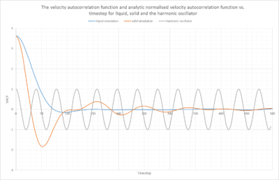
The VACF autocorrelation functions contain information about the dynamic fluctuations for self-diffusion. The VACF "defines the projection in time of the particle's velocity along its initial direction."[2] The time dependent variation "offers a wealth of information about the microscopic motions underlying the dynamical behavior of the fluid."[2] The liquid and the solid VACF decay in the first region, meaning at the shortest times, this slow decay of the VACF is called the "free flight", because the particle's velocity remains at its initial value."[2]This free flight part is slightly longer for the liquid, because the density is lower and therefore it takes longer until the particles in the liquid encounter other particles than for the solid case.

However, once they start colliding, the second region is reached, at short to moderate times, the VACF now "decays quickly due to the onset of collisions with surrounding particles"[2]. The solid VACF decays more steeply due to the higher density and the larger amount of particles in close proximity to collide with. Thus, the minimum for the solid VACF is much more negative and occurs earlier than in the solid example. Note that these minima are negative due to the back scattering effect, meaning that the collision of the particles causes them to change direction, resulting in a negative VACF. The minimum is the turning point, the point at which the previous velocities stop being correlated.

In the third region, which occurs at long times, the VACF goes to zero $C(\tau )=0$, indicating the absence of any residual correlation. Strictly speaking, this is only true for the liquid, the solid VACF still fluctuates a lot around zero due to the vibrations inside the solid.

Harmonic oscillator VACF vs. the Lennard Jones solid and liquid

The harmonic oscillator can be understood as a spring, that bounces back and forth between two fixed points (1/-1 and 0, indicating full correlation), this is why we observe this periodical behaviour. Starting at 1 on the harmonic oscillator VACF, once the particle moves a bit further in a small number of timestep we would measure a VACF number slightly smaller than 1. Thus, with each movement of the particle in the direction v. The VACF correlation decreases, since the particle is increasing its difference to the starting position. Once it reaches the "end", meaning the fixed point were the springs feels a resistance and bounces off to the other side. This point is 0 on the VACF graph, since this is the least correlated we can get to in a harmonic oscillator. Once it has reached this point, it changes direction and goes back along the same way it came, now travelling at a negative velocity -v. This is why the VACF values are negative. They become closer and closer again to their starting point, therefore the correlation increases from 0 to -1. -1 indicating the starting point, the point of 100 % correlation and this continues to infinity as we assume ideal conditions and constant total Energy. Therefore the movement of the harmonic oscillator remains correlated.

For the Lennard Jones liquid and solid, the particles are initially kept in a solvation shell or a lattice, which is why we initially observe a controlled movement similar to the harmonic oscillator. The VACF starts at a maximum indicating full correlation, similiar to 1 in the harmonic oscillator. However these functions have not been normalised. If they were, they would start at 1. The particle vibrates and it hits one of the particles next to it in the solvation shell/lattice, this is when it passes through zero, and it reaches no correlation. The particle then bounces back in the direction it came from, similar to the harmonic oscillator, leading to an increase in correlation until it reaches the starting point, full correlation. If they were normalised this would tend towards -1. However, the particle does not just stop at its starting point, after bouncing back, it leaves the solvation shell and escapes, resulting in a multitude of collisions, which decrease the correlation and result in random behaviour, in other words, the VACF graph goes to zero.

NJ: The key reason the HO doesn't decorrelate is that there is nothing for it to collide with. Otherwise, this is an excellent description, well done.

Task 4

Fig.19 VACF vs. Time for a gas (8000 atoms) Fig. 20 Running Integral vs. Time for a gas (8000 atoms)

Fig.21 VACF vs. Time for a gas (1 million atoms) Fig. 22 Running Integral vs. Time for a gas (1 million atoms)

Fig.23 VACF vs. Time for a liquid (8000 atoms) Fig. 24 Running Integral vs. Time for a liquid (8000 atoms)

Fig.25 VACF vs. Time for a liquid (1 million atoms) Fig. 26 Running Integral vs. Time for a liquid (1 million atoms)

Fig.27 VACF vs. Time for a solid (3200 atoms) Fig. 28 Running Integral vs. Time for a liquid (3200 atoms)

Fig.29 VACF vs. Time for a liquid (1 million atoms) Fig. 30 Running Integral vs. Time for a liquid (1 million atoms)

Description Gas

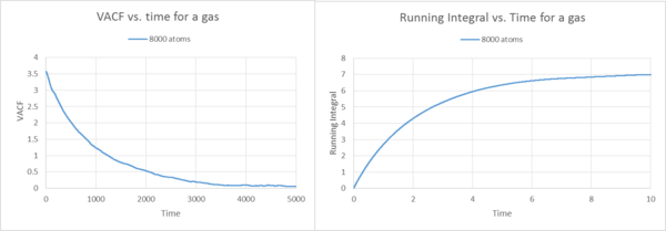
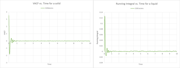
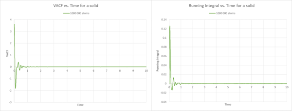
By using the trapezium rule, the running integrals were plotted against time, based on the VACF functions. These integrals show what we would expect. The VCAF is the same as before for the liquid and solid 8000 atoms case. In the liquid example the running integral builds up by adding tiny trapezes together over time. Therefore the running integral plot starts at zero for the gas and then builds up rapidly, because if we look at the VACF plot, at the start is where we should find the biggest area under the curve, as time elapses, the VACF decreases, thus the area underneath the graph decreases. Therefore by adding the trapezes to the running integral, the level off because the area only builds up by tiny amounts if you have reached approximately 8 seconds. This observation is the same for the 1000 000 atoms gas running integral plot. However, the 1000 000 atoms plot shows a gradual increase, not as steep as for the 8000 atoms. Generally speaking, it is a more precise representation and therefore levels off less quickly.

For the gas, no matter if 8000 or 1 000 000 atoms, we observe the highest diffusion coefficients, thus by far the highest running integrals (note the difference in scale). Therefore the graph, plateaus off later than for the liquid or the solid.

Description Liquid

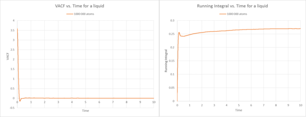
By comparing the VACF plots for the liquid with 8000 atoms and 1000 000 atoms, we observe that they are quite similar, and that the fluctuations around VACF=0 are less visible at higher atom sizes (1000 000 atoms). This shows that with increasing number of atoms, the correlation tends to zero. Thus, for an infinite number of atoms, the correlation is zero. The initial trend towards the minimum has been described in the previous task and is due to the controlled movement inside the solvation shell. For the running integrals, they reflect the development of the area underneath the curve, at the start we observe the biggest increase in the integral.

The diffusion constants are very similar for 8000 and 1000 000 atoms. These constants are smaller than for the gas, because there is higher frictional force due to the higher density of the state, inhibiting diffusion. This constant is hence bigger than for the solid, because in the solid the atoms remain in their lattice structure.

Description Solid

The VACF plots for the solid are what I would expect because, we observe the initial non-normalised oscillator like movement described in the question above. However, when reached the minimum, the VACF becomes only less correlated and fluctuates around VACF=0 for 3200 atoms. When the number of atoms is increased, this behaviour is even more apparent, due to the fact that we observe an almost straight line along VACF=0, indicating non-correlated random behaviour. If we now compare the VACF with the respective running integral plots, we note the similar trend as observed for the gas. In the running integral plot, the area increases by the largest amount at the start, because before VACF reaches zero for the first time, we observe the largest area under the VACF curve. Then it quickly fluctuates around zero and therefore the area tends to zero. This is true for both sets of atoms. Due to the higher degree of order and the vibrations around 0, the area is much smaller than for the liquid example. This is coherent with the fact that the diffusion constant for the solid is significatnly smaller than for the liquid. When looking at the diffusion coefficients, $D_{1000000}$ is slightly smaller than $D_{3200}$, due to the fact that if the set of atoms is much bigger, the atoms have more trouble to move, because there is a higher probability that they collide with each other.

The diffusion constant for only 3200 atoms seems to be slightly off the 1000 000 atoms set, this may be due to the smaller set of atoms. We have seen from previous questions and the liquid and gas example, that the values become more precise as we increase the set of atoms.

THE DIFFUSION CONSTANTS OBTAINED BY USING THE RUNNING INTEGRALS

$D=\frac{1}{3}\underset{0}{\overset{\mathrm{\infty }}{\int }}\mathrm{d}\tau ⟨\mathbf{v}\left(0\right)\cdot \mathbf{v}\left(\tau \right)⟩$

Thus: The last running integral has to be used, because it incorporates all previously calculated integrals. This last running integral has to be divided by 3 to obtain the diffusion coefficient.

The diffusion coefficients are therefore:

Gas:

$D_{8000}=2.33m^2{s}^{-1}$

$D_{10000000}=3.27m^2{s}^{-1}$

Liquid

$D_{8000}=9.7910^{-2}{m}^2{s}^{-1}$

$D_{10000000}=9.0110^{-2}{m}^2{s}^{-1}$

Solid

$D_{3200}=1.8410^{-04}$

$D_{1000000}=4.5529510^{-05}$

NJ: These are still dimensionless!

The largest source of error in your estimates of D from the VACF

A possible source of error must be, that we rely on the VACF to calculate D and VACF gains accuracy by increasing the number of atoms. This must be the largest source of error, because when we compare the D constants with the ones calculated using MSD, for the gas and liquid, the constants are of the same order of magnitude. Only for the solid, we notice a bigger discrepancy.

However, the biggest source of error should be the fairly simplistic way of calculating the areas by using the trapezium rule. There are more advanced mathematical integration methods that would lead to better results. The trapezium rule would become a better approximation if the timestep ie. the difference between the times was decreased. If we cut down the intervals into an infinitesmal size, we would get the best result.

References

[1] 411-506 Computational Physics 2 4 Wednesday, January 16, 2013, Topic 1 Molecular Dynamics Lecture 2, http://www.physics.buffalo.edu/phy411-506/topic1/topic1-lec2.pd

[2]http://turbo.che.ncsu.edu/smithsw/paper1/node10.html

[3]http://www.csb.yale.edu/userguides/datamanip/autodock/html/Using_AutoDock_305.a.html#29613

[4]http://www.chem.iitb.ac.in/~bltembe/pdfs/lect11.pdf