Talk:Mod:Gcf14

JC: The data looks good and report is well laid out and clear. There were a few mistakes towards the beginning, especially on the background theory so make sure you understand this and a few explanations lacked a bit of detail.

Theory

In this experiment, the simulations are run using the velocity-Verlet algorithm.

The velocity-Verlet algorithm was used to model a harmonic oscillator. The results of this are shown in figures 1-4.

Figure 1: A plot of the output of the velocity-Verlet algorithm

Figure 2: A plot of the absolute error for the energy

Figure 3: A plot showing the energy at a timestep of 5

Figure 4: A plot showing the energy at a timestep of 0.3

The timestep of the model was changed, to see the effect it had on the energy of the system. As the timestep increased, the energy had a large change over the course of the simulation. An example of this is shown in figure 3. In order for the energy to not change by more than 1% over the course of the simulation, a timestep in the order of 0.2-0.3 needed to be used. An example of this is shown in figure 4. It is important to monitor the total energy when modelling its behaviour numerically because the total energy should remain constant. Therefore, it is a good indication as to how good the simulation is; if the energy fluctuates a lot, the simulation is not as good.

JC: The results in fig 1 and 2 look good, but why does the energy fluctuate around 0 in fig 3 and 4, are you plotting the total energy or just the kinetic or potential component?

Atomic Forces

A single Lennard-Jones interaction can be described using the following equation:

$\varphi (r)=4ϵ(\frac{{\sigma }^{12}}{r^{12}}-\frac{{\sigma }^6}{r^6})$

The separation of two atoms where the potential energy is equal to zero can be found by setting the equation above equal to 0 and rearranging to find r.

$4ϵ(\frac{{\sigma }^{12}}{r^{12}}-\frac{{\sigma }^6}{r^6})=0$

$\frac{{\sigma }^{12}}{r^{12}}=\frac{{\sigma }^6}{r^6}$

$r=r_0=\sigma$

Once $r_0$ has been found, this value of r can be substituted back into the original equation for $\varphi (r)$ to find the force at this separation. At this value of r, the force = 0.

JC: $\varphi (r)$ is the potential, not the force - to calculate the force you need to differentiate $\varphi (r)$.

The equilibrium separation, $r_{eq}$, can be found by differentiating the original equation for the Lennard-Jones potential with respect to r.

$\frac{d\varphi (r)}{d(r)}=4ϵ(\frac{-12{\sigma }^{12}}{r^{11}}+\frac{6{\sigma }^6}{r^5})$

When this differential is set to zero, the value of $r_{eq}$ is then be found by rearranging the equations, the result of which is shown below.

$0=4ϵ(\frac{-12{\sigma }^{12}}{r^{13}}+\frac{6{\sigma }^6}{r^7})$

$\frac{6{\sigma }^6}{r^7}=\frac{12{\sigma }^{12}}{r^{13}}$

$r^6=2{\sigma }^6$

$r_{eq}=2^{\frac{1}{6}}\sigma$

Having found the value of $r_{eq}$, the force at this separation could be found, by substituting in this value back into the original equation.

$\varphi (r)=4ϵ(\frac{{\sigma }^{12}}{(2^{\frac{1}{6}}\sigma {)}^{12}}-\frac{{\sigma }^6}{(2^{\frac{1}{6}}\sigma {)}^6})$

$\varphi (r)=4ϵ(\frac{1}{4}-\frac{1}{2})$

The energy at this separation, and therefore the depth of the potential well, is equal to $-ϵ$.

The following integrals were then evaluated:

$\underset{2\sigma }{\overset{\mathrm{\infty }}{\int }}\varphi (r)dr,\underset{2.5\sigma }{\overset{\mathrm{\infty }}{\int }}\varphi (r)dr,\underset{3\sigma }{\overset{\mathrm{\infty }}{\int }}\varphi (r)dr$

The general result from integrating the function for $\varphi (r)$ is:

$\int \varphi (r)dr=4ϵ(\frac{{\sigma }^6}{5r^5}-\frac{{\sigma }^{12}}{11r^{11}})+c$

When evaluated using the limits above, the results are:

$\underset{2\sigma }{\overset{\mathrm{\infty }}{\int }}\varphi (r)dr=-0.0248$ $\underset{2.5\sigma }{\overset{\mathrm{\infty }}{\int }}\varphi (r)dr=-0.00818$ $\underset{3\sigma }{\overset{\mathrm{\infty }}{\int }}\varphi (r)dr=-0.00329$

Periodic Boundary Conditions

The number of water molecules in 1 mL of water under standard conditions can be estimated using the following equation.

$pV=N{k}_{B}T$

Where:

• $p$ is the pressure ( = 101.395 kPa)

• $V$ is the volume in $m^3$

• $N$ is the number of molecules

• $k_B$ is the Boltzmann constant ( = $1.38064852{\times }^{-23}$)

• $T$ is the Temperature under standard conditions ( = 298.15 K)

The number of molecules in 1 mL was estimated to be $2.46\times 10^{19}$ molecules. In addition, the volume of 10000 molecules was also estimated. It was found to be $4.0625\times 10^{-22}{m}^3$.

JC: Under standard conditions the density of water is 1g/ml, the ideal gas law will give a poor estimate of the density of liquid water.

For the number of molecules in the box to remain constant, if a particle exits the box on one side, it reappears on the opposite face. For example, if a particle starts at $(0.5,0.5,0.5)$ in a cubic box which runs from $(0,0,0)$ to $(1,1,1)$ and moves along the vector $(0.7,0.6,0.2)$, the particle ends up in position $(0.2,0.1,0.7)$ once the periodic boundary conditions have been applied.

JC: Correct.

Reduced Units

Reduced units are used to make the values more manageable. For example, $r$ in reduced units becomes $r^{*}=\frac{r}{\sigma }$

Therefore, in the case of $r^{*}$ equaling 3.2, r would be $1.088\times 10^{-9}$. The well depth in this case would be 0.998 $kJmo{l}^{-}1$

For a reduced temperature, $T^{*}$, of 1.5, the temperature in real units is 180 K. This was found by rearrangement of the equations below:

$T^{*}=\frac{k_{B}T}{ϵ}$ and $\frac{ϵ}{k_B}=120K$

Equilibration

The simulations work by specifying the starting points of the atoms and then allowing the simulation to run.

If the starting coordinates given to the atoms are random, and two end up too close to each other, then there are very large repulsive forces, which causes the simulation to breakdown. Therefore, the initial start point is based off of a lattice.

For these simulations, the density of lattice points has been set to 0.8. As the mass of the atoms has been set equal to 1, the volume of the simulation box can be calculated using $Density=\frac{mass}{volume}$. In this case, the volume is 1.25. From this, the length of the side of the cell can be found, and is 1.07722.

If the cell were a face-centred cubic lattice, as opposed to a simple cubic lattice, with a density of 1.2, the length of the side of the cell can be found to be 0.941.

JC: How did you calculate this, the side length should be the cube root of (4/1.2) = 1.49 for an fcc lattice.

If this lattice had been defined as a face centred cubic lattice instead of the simple cubic lattice, the number of atoms created would have been 4000. This is because instead of having 1 atom per unit cell, there are 4, as a result of having more lattice points. In the simple cubic cell, there is a lattice point on each corner of the cube. These contribute $\frac{1}{8}$ to the overall number of lattice points, as they are shared by 8 unit cells. However, in the case of the face-centred cubic lattice, there are these lattice points on the corners, as well as 1 lattice point per face, which contributes 0.5 as it shared by 2 unit cells. Therefore, due to a cube having 6 faces, there are 3 extra lattice points, resulting in 4 overall.

LAMMPS Manual

mass 1 1.0
pair_style lj/cut 3.0
pair_coeff * * 1.0 1.0

The purpose of the mass command is to set the mass of all of the atoms. In this case it is setting the mass of the atoms which are of type 1 to a value of 1.0.

The purpose of the pair_style command is to set the formula that the LAMMPS software uses to compute the pairwise interactions. In this case, lj means refers to Lennard-Jones, and the cut means there is a cutoff at an r value of 3.0 in reduced units.

The purpose of the pair_coeff command is to set the force field coefficients for the atom types.

JC: What are the force field coefficients in this case, with a Lennard- Jones potential?

### SPECIFY TIMESTEP ###
variable timestep equal 0.001
variable n_steps equal floor(100/${timestep})
variable n_steps equal floor(100/0.001)
timestep ${timestep}
timestep 0.001

### RUN SIMULATION ###
run ${n_steps}
run 100000

The purpose of writing this, as opposed to just having a command setting the timestep and then to run it, is so that the timestep can be easily changed. In addition, it is so that the right number of readings are taken, as the first run is dependent upon n_steps, which is related to the timestep (shown in the fourth line).

JC: Correct, using variables makes it much easier to change one property of a simulation without having to manually change ever line in the simulation script that depends on that property.

Integration algorithm

Because we have specified both the position and the velocity, we are going to use the velocity-verlet algorithm.

The first simulation

For the first set of simulations, the timestep was varied in order to find out the optimal timestep to use in future simulations. The timesteps used were: 0.001 s, 0.0025 s, 0.0075 s, 0.01 s and 0.015 s.

The data was then plotted, and these graphs are shown below.

Figure 5: A graph of total energy against time for the 0.001 timestep

Figure 6: An expansion in the x region 0-5 s for the graph of total energy against time for the 0.001 timestep

Figure 7: A graph of pressure against time for the 0.001 timestep

Figure 8: A graph of temperature against time for the 0.001 timestep

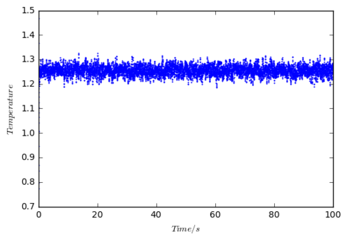
For the 0.001 timestep, the simulation reaches equilbrium. This occurs after approximately 0.58 seconds.

Figure 9: A graph of total energy against time for all of the 5 timesteps simulated

Figure 10: An expansion in the region 0-x s for the graph of total energy against time for all of the 5 timesteps simulated

Figures 5 and 6 have the total energy vs time plotted for the 5 timesteps used. From these graphs we can choose a suitable timestep for the later simulations. The timestep chosen was 0.0025. The reason for choosing this timestep is that it was only one of two that reached convergence within the time limit. These two timesteps were 0.0025 and 0.001. The reason why 0.0025 was chosen, is that it is the larger of the two that reached convergence, and therefore was a better choice due to computational efficiency. The 0.15 timestep was an obviously bad choice, because instead of converging, it diverged.

JC: Correct, total energy should be independent of the timestep.

Running Simulations Under Specific Conditions

Thermostats and Barostats

The temperature and pressure need to be maintained at values near the target values. For temperature this is achieved by multiplying the velocities of the particles by a factor, $\gamma$, which alters the instantaneous temperature, T, so that it is closer to the target temperature, $\mathfrak{𝔗}$.

For the simulated system, the equation below relates the classical equation for Kinetic energy to the kinetic energy equation found from equipartition theorem.

$\frac{1}{2}\sum _i{m}_{i}v{i}^2=\frac{3}{2}N{k}_{B}T$

As mentioned previously, when the temperature fluctuates from the target temperature the velocities are multiplied by a factor $\gamma$. The result of this is shown in the equation below.

$\frac{1}{2}\sum _i{m}_i(\gamma vi{)}^2=\frac{3}{2}N{k}_B\mathfrak{𝔗}$

The two above equations can then be manipulated and equated to find an expression for the value of $\gamma$. This is shown in the equations below.

$({\gamma }^2)\frac{1}{2}\sum _i{m}_{i}v{i}^2=\frac{3}{2}N{k}_B\mathfrak{𝔗}$

$({\gamma }^2)\frac{3}{2}N{k}_{B}T=\frac{3}{2}N{k}_B\mathfrak{𝔗}$

${\gamma }^2=\frac{\mathfrak{𝔗}}{T}$

JC: Correct and well laid out.

A similar principle is used to maintain the pressure near the target pressure. If the pressure is too large, then the volume of the simulation box increases whereas if the pressure is too small, the volume of the simulation box decreases.

In the input script, the following commands are used.

fix aves all ave/time 100 1000 100000 ...

The 100 is the value of Nevery, which relates to the how often a value is inputted. So in this example, a value is inputted every 100 timesteps. 1000 is the value of Nrepeat. This means that 1000 values of timestep as used to calculate each average. 100000 is Nfreq, and it means that the programme calculates an average this many timesteps.

Running Simulations Under Specific Conditions

In this section, the simulations that were run were done under varying conditions. Overall, ten simulations were run at two different pressures, 2.6 and 2.9. These were chosen based off of the graph of average pressure throughout the simulation (firgure 7). The simulations were run at 5 different temperatures for each pressure. These were: 1.6, 1.8, 2.0, 2.2 and 2.4.

The results of these simulations are plotted on the graph below.

Figure 11: A graph plotting density as a function of temperature for pressures of 2.6 and 2.9.

Figure 12: A graph plotting density as a function of temperature for the simulated and theoretical results

The result was as expected, as the higher pressure led to a higher density. In addition, the lower the temperature, the higher the density. Both of these results were expected. A line was then plotted based on the ideal gas law, and is shown in figure 12.

The theoretical results gave a higher density than the simulated result; this is as a result of collisions which occur in the simulation, which are not taken into account in the theoretical results. Also the discrepancy between the simulated and the theoretical results increased at higher pressures.

JC: Error bars look good. It is misleading to join data points by straight lines though, as in the ideal gas results in fig 12, since this is not what's predicted by the ideal gas law. The reason that the ideal gas and simulation results don't agree is the lack of any interactions in the ideal gas law. Why does the discrepancy increase with pressure and decrease with temperature?

Calculating Heat Capacities using Statistical Physics

In this section, simulations were ran at 10 points and at two different densities (0.2 and 0.8). For each density, the simulations were run at 5 temperatures (2.0, 2.2, 2.4, 2.6 and 2.8).

The results of the simulation were then plotted as $\frac{C_V}{V}$ against temperature. The volume of the box was found by using the equation $density=\frac{mass}{volume}$, and the fact that the mass of the atoms was set to 1. Therefore, the volume was simply 1/density.

Figure13: A graph plotting $\frac{C_V}{V}$ as a function of temperature.

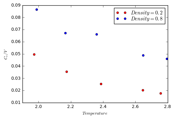
The expected trend is that the heat capacity will increase with temperature. However, this is not the case based on the results from the simulation. A possible reason for this could be due to the fact that the simulation is based on a lattice. Therefore, there is no way for the atoms to undergo rotational motion (there are fewer degrees of freedom). The result of this is that the increase in temperature leads to a decrease in the heat capacity.

JC: Why do you expect heat capacity to increase with temperature? The atoms in this simulation are spherical and so have no rotational degrees of freedom.

For this simulation, the input script had to be edited as a result of changing ensemble from npt to nvt, as well as needing to have a density variable. An example of the input script is shown below.

	GCF14nvt0.2.2.8.in

File:GCF14nvt0.2.2.8.in

Structural Properties and the Radial Distribution Function

RDF's

Radial Distribution functions give information on how particles are packed around a reference particle. Therefore, they can be used to elucidate the structural features of the simulated system.

To calculate the RDF's of the three phases, simulations were run in each phase, and the trajectories were then used to calculate the RDF's. Suitable temperatures and densities for the simulation were found here[2]

Figure 14: A graph of the RDF's of the simulated gas, liquid and solid system.

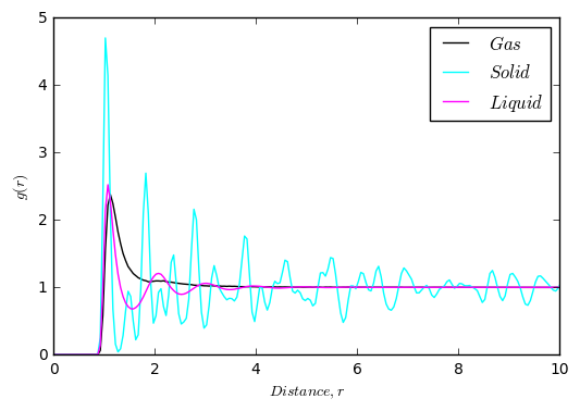
As can be seen from the plots above, the RDF's are all vastly different. The area under the curve is the probability of finding a particle at that distance from the reference particle. For the gas RDF, there are very few features. The reason for this is that the particles are very spread out, and so there is little probability of finding another particle.

Liquids are more ordered than gases, as they have coordination spheres. This is shown in the RDF by a series of peaks of decreasing height. It shows that there is a reasonable probability of finding another particle in the primary coordination sphere, but as you go further away from the reference particle this probability decreases.

Solids are in a lattice, and so the positions of the particles are somewhat fixed. Therefore, there are several peaks in the RDF corresponding to neighbouring atoms. This is also the reason why the peaks are broad, as the atoms are vibrating about a fixed position. Each peak represents a coordination shell. The first peak corresponds to the first set of nearest neighbours, shown in orange on the diagram. The second maxima corresponds to the second set of nearest neighbours shown in green, and the third maxima corresponds to the third set, shown in yellow.

The lattice spacing was found to be 1.625.

Figure 15: A diagram to show the nearest neighbours in a FCC lattice

The coordination number can be elucidated from the plot of integration of g(r).

Figure 16: A plot of r vs g(r)

The coordination number of the first peak (at approx. 1.225) is 12. The coordination number of the second peak (at approx. 1.625) is 6. The integration is 18, and so there are 6 coordination sites. The coordination number of the third peak (at approx. 1.975) is 24. This results from the integral being 42. This number of coordination sites makes sense, as there are 3 neighbours, and 8 unit cells, resulting in a coordination of 24.

JC: How did you calculate the lattice spacing, did you try calculating it from the first or third peak in the RDF so that you could take an average? Good idea to use a diagram to show the nearest neighbours.

Dynamical Properties and the Diffusion Coefficient

Simulations were run at a specified denisty and temperature in order to find the mean squared displacement. This enables us to find out how much the atoms move during the simulation, and subsequently the diffusion coefficient.

The graphs below plot the results of these simulations.

Figure 17: A graph of total mean squared displacement against timestep for a gas.

Figure 18: A graph of total mean squared displacement against timestep for a liquid.

Figure 19: A graph of total mean squared displacement against timestep for a solid.

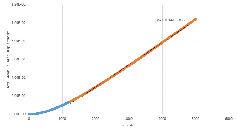
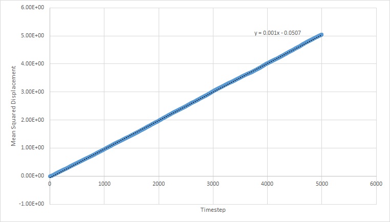
The equation for the diffusion coefficient is $\frac{1}{6}\frac{\delta <r^2(t)>}{\delta t}$. From the graphs, the diffusion coefficient can be estimated, as it is the gradient of the linear part of the graph divided by 6. The values for D are as follows (in reduced units):

$GasD=0.00407$

$LiquidD=0.000167$

$SolidD=16.7\times 10^{-9}$

This was then repeated on the supplied data (simulation with one million atoms). These graphs are shown below.

Figure 20: A graph of total mean squared displacement against timestep for a gas (1 million atoms).

Figure 21: A graph of total mean squared displacement against timestep for a liquid (1 million atoms).

Figure 22: A graph of total mean squared displacement against timestep for a solid (1 million atoms).

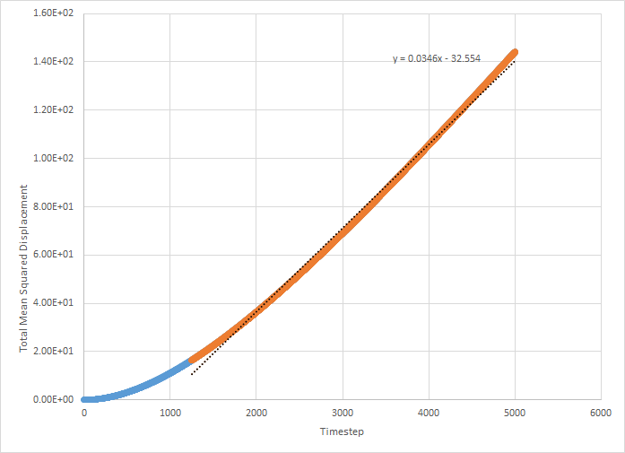
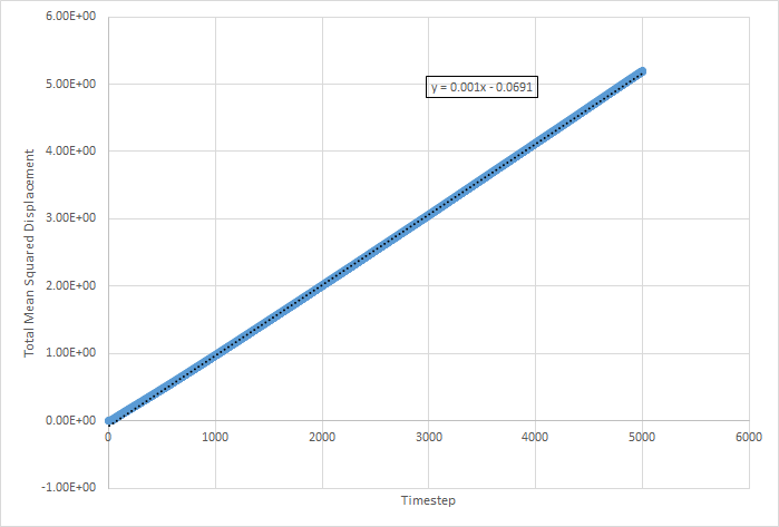
The values for D for the million atoms simulation are as follows:

$GasD=0.00576$

$LiquidD=0.000167$

$SolidD=16.7\times 10^{-9}$

For the solid MSD graphs, after the system has reached equilibrium, the diffusion coefficient is close to zero. The reason for this is because the atoms are almost fixed as a result of being in a lattice and therefore cannot move. For a liquid, the graph is linear, because of the collisions which occur between the molecules as they move, which results in linear diffusion. For the gas, the graph starts off as ballistic motion, where the molecules travel without colliding as a result of the molecules being so far apart. This is why it starts of curved, as the ballistic motion is proportional to $T^2$. When the molecules start colliding, the graph becomes linear, as it undergoes linear diffusion. The diffusion coefficient was found to be greatest for a gas, which is expected.

JC: Good explanation of the shapes of the 3 graphs. Make sure you only use the linear section of the mean squared displacement graph to calculate the diffusion coefficient for the gas.

Finding the Diffusion coeffcient by integration

By evaluating the integral of $C\left(\tau \right)$, the diffusion coefficient can also be estimated. This is as a result of the following equation:

$D=\frac{1}{3}\underset{0}{\overset{\mathrm{\infty }}{\int }}\mathrm{d}\tau ⟨\mathbf{v}\left(0\right)\cdot \mathbf{v}\left(\tau \right)⟩$

whereby $⟨\mathbf{v}\left(0\right)\cdot \mathbf{v}\left(\tau \right)⟩$ is equal to $C\left(\tau \right)$.

The following is the evaluation of this integral.

$x(t)=Acos(\omega t+\varphi )$

$v(t)=\frac{dx(t)}{dt}=-A\omega sin(\omega t+\varphi )$

$C\left(\tau \right)=\frac{\underset{-\mathrm{\infty }}{\overset{\mathrm{\infty }}{\int }}v\left(t\right)v(t+\tau )\mathrm{d}t}{\underset{-\mathrm{\infty }}{\overset{\mathrm{\infty }}{\int }}{v}^2\left(t\right)\mathrm{d}t}$

$C\left(\tau \right)=\frac{A^2{\omega }^2\underset{-\mathrm{\infty }}{\overset{\mathrm{\infty }}{\int }}sin(\omega t+\varphi )sin(\omega (t+\tau )+\varphi )dt}{A^2{\omega }^2\underset{-\mathrm{\infty }}{\overset{\mathrm{\infty }}{\int }}si{n}^2(\omega t+\varphi )dt}$

$where{A}^2{\omega }^2\underset{-\mathrm{\infty }}{\overset{\mathrm{\infty }}{\int }}sin(\omega t+\varphi )sin(\omega (t+\tau )+\varphi )dt=INTEGRAL1$

$where{A}^2{\omega }^2\underset{-\mathrm{\infty }}{\overset{\mathrm{\infty }}{\int }}si{n}^2(\omega t+\varphi )dt=INTEGRAL2$

Focusing on Integral 1....

Integral 1 = $\int sin(\omega t+\varphi )sin(\omega t+\varphi )cos(\tau )+sin(\omega t+\varphi )sin(\tau )cos(\omega t+\varphi )dt$

which gives.... $\frac{cos(\tau )}{2}(t-\frac{1}{2\omega }sin(2(\omega t+\varphi )))+sin(\tau )\int sin(\omega t+\varphi )cos(\omega t+\varphi )dt$

Integral 3 = $\int sin(\omega t+\varphi )cos(\omega t+\varphi )dt$

Solve Integral 3 by substitution....

$u=sin(\omega t+\varphi )$

$\frac{du}{dt}=\omega cos(\omega t+phi)$

$\frac{1}{\omega }du=cos(\omega t+\varphi )dt$

$=\frac{sin(\tau )}{\omega }\int udu$

$=\frac{sin(\tau )}{2\omega }si{n}^2(\omega t+\varphi )$

Therefore, integral 1 = $\frac{cos(\tau )}{2}(t-\frac{1}{2\omega }sin(2(\omega t+\varphi )))+\frac{sin(\tau )}{2\omega }si{n}^2(\omega t+\varphi )$

Going back to integral 2:

Integral 2 = $\underset{-\mathrm{\infty }}{\overset{\mathrm{\infty }}{\int }}si{n}^2(\omega t+\varphi )dt$

which $=\frac{1}{2}(t-\frac{1}{2\omega }sin(2(\omega t+\varphi )))$

Therefore, combining integrals 1 & 2 gives:

$\frac{\frac{cos(\tau )}{2}(t-\frac{1}{2\omega }sin(2(\omega t+\varphi )))+\frac{sin(\tau )}{2\omega }si{n}^2(\omega t+\varphi )}{\frac{1}{2}(t-\frac{1}{2\omega }sin(2(\omega t+\varphi )))}$

Which when evaluated using the limits simplifies to:

$C\left(\tau \right)=cos(\omega \tau )$

JC: How do you evaluate the last expression using the limits to get to the answer? You don't actually need to perform any integration if you split up the numerator into a sin squared term which cancels with the denominator and a sin x cos term that is an odd function and so integrates to zero (if limits are placed symmetrically about zero). Include a few more steps to make your derivation clearer.

Using the evaluated Integral

Figure 23: A graph plotting cos(wt) vs tau for a harmonic oscillator, VACF for solids and liquids.

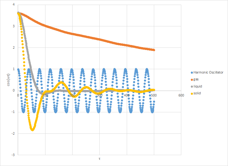
The graph shows plots of a harmonic oscillator and the VACF plots for a solid (yellow) and liquid (grey). The minima represent particles oscillating in the opposite direction to tau, therefore causing the negative minima. Eventually, these oscillations are no longer in phase, and so cancel out. This is the reason why they converge.

The graph for the harmonic oscillator is very different. The reason for this is because we are modelling a single particle, and so there are no collisions which would cause it to converge to zero.

The trapezium rule was then used to integrate to find the area under the curve. The reason for doing this is that it allows you to estimate the value for the diffusion coefficient.

Plots of the running integral for the simulation are shown below.

Figure 24: A graph plotting the running integral vs time for a gas

Figure 25: A graph plotting the running integral vs time for a liquid

Figure 26: A graph plotting the running integral vs time for a solid

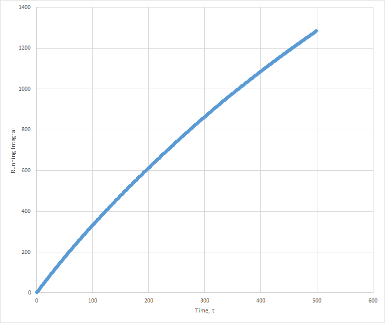
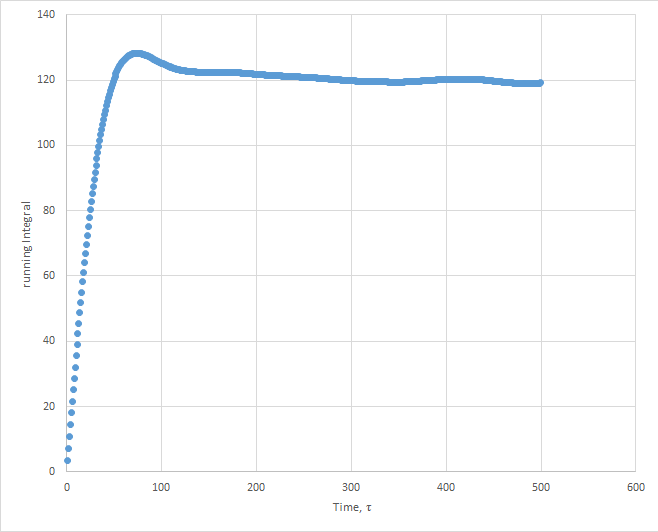
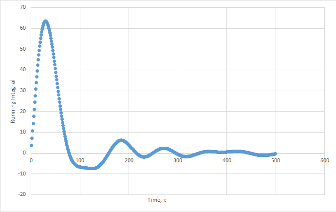
The values of D estimated from the Trapezium rule are: Solid D = -0.127 , Liquid D = 39.7 , Gas D = 428 .

This was then repeated using the files from the 1 million atom simulation, which gave the following D values: Solid D = -1.33, Liquid D = 40, Gas D = 488.

Figure 27: A graph plotting cos(wt) vs tau for a harmonic oscialltor, VACF for solids and liquids (1 million atoms sim).

Figure 28: A graph plotting the running integral vs time for a gas (1 million atoms sim)

Figure 29: A graph plotting the running integral vs time for a liquid (1 million atoms sim)

Figure 30: A graph plotting the running integral vs time for a solid (1 million atoms sim)

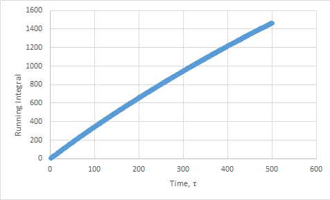
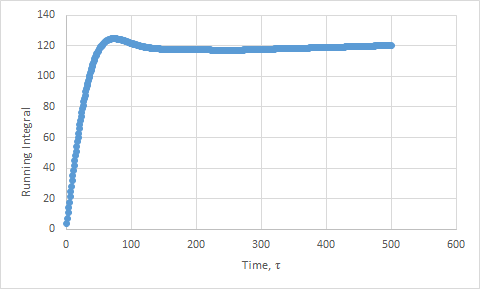
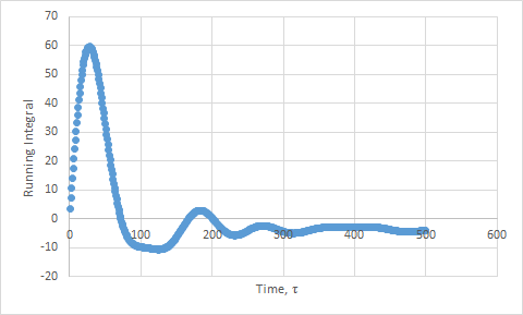
The values of D for the integration method showed the same trend as the previous method. However, the values are slightly higher than expected, due to the approximation not being as good. We have assumed that the velocities do not change upon collisions. This is a poor assumption to make. In addition, the trapezium rule adds in more error.

JC: When do you assume that the velocities don't change upon collision? Do you think that the diffusion coefficient can be estimated from the running integral for the gas if the curve hasn't flattened out?

References

- ↑ LAMMPS Manual, http://lammps.sandia.gov/doc/Section_commands.html#lammps-input-script , accessed November 2016
- ↑ JP Hansen, L Verlet, Phys Rev, 184, 1969, http://journals.aps.org/pr/abstract/10.1103/PhysRev.184.151
- ↑ Diagram of FCC Lattice, adapted from http://ecee.colorado.edu/~bart/book/bravais.htm , accessed November 2016