Talk:Mod:FRMD

JC: General comments: All tasks completed and results well presented. Some of the written explanations were a bit confusing though, make sure that you understand the background theory behind each task so that you can fully explain what your results show and what they mean physically.

Introduction

Molecular dynamics can be used in many situations where a real life experiment may not be feasible. Being able to run highly sophisticated computer simulations can provide an insight into a wide range of real life systems, and to remarkable accuracy. It can be used to calculate the position, velocity and appropriate force of an atom to measure thermodynamic properties such as a system's energy, volume, heat capacity and temperature, all from the comfort of a desk, and without the need to ever wear a lab coat. The core principle behind it is the solving of Newton's equations of motion for a system of interacting particles, at a snapshot in time. These are dependent on a previous conditions, and these snapshots are built up to form an overall picture. Statistical physics enables us to take all the individual properties and combine them, to form a replica of a real life system.

For this experiment, the Large-scale Atomic/Molecular Massively Parallel Simulator, or LAMMPS software was used. After optimising the accuracy of the simulation, density, heat capacity and diffusion coefficient were investigate, for solid, liquid and vapour states.

Introduction to molecular dynamics simulation

The velocity verlet algorithm considers the acceleration of an atom to be dependent on its position, and was used to calculate the velocities and positions at snapshots in time.

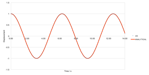
Initially, we used this algorithm to model a simple harmonic oscillator. To assess it's accuracy, a classical simple harmonic oscillator was also modelled, and the position of an atom from this model is shown in equation 1. For our calculations, $$\begin{gathered} \varphi =0 \\ A=1.00 \\ \omega =1.00 \end{gathered}$$. The total energy was calculated from the sum of the kinetic and potential energy, shown in equation 2.

$$\begin{gathered} x(t)=A\cos (\omega t+\varphi ) \\ (1) \end{gathered}$$ $$\begin{gathered} E=K+U=\frac{1}{2}m{v}^2+\frac{1}{2}k{x}^2 \\ (2) \end{gathered}$$

For a timestep of 0.1s, the two models are shown in figure 1. The error between the two models is shown in figure 2, and the maxima can be connected using a linear fit, of equation $4.21552195\times 10^{-4}x-7.3021874\times 10^{-5}$.

Figure 1. Displacement vs time using the velocity-varlet algorithm

Figure 2. The absolute error between the classical solution and the velocity-varlet solution

The simulation occurs over the course of 100s, meaning the error is much larger towards the end of the simulation, due to the error being a function of time. Figure 3 shows the maximum errors associated with several time steps, and shows a dramatic enhancement in the accuracy of the model by reducing the time step by a factor of 10. This results in a reduction in absolute error by a factor of 100.

Figure 3. Absolute error for several time steps

The total energy of the system also oscillates slightly, as shown in figure 4. As the system is meant to be isolated, the total energy should remain constant and so it is important to monitor the total energy to ensure the model is representative of the real life situation it is trying to replicate. These oscillations can be reduced by reducing the time between the measured snapshots, as the velocity verlet algorithm endures an error in the calculation of the position and velocity. This is due to both calculations involving the multiplication of a previously calculated value by the $\delta t$. The error for the algorithm for position can be derived to be $O(\mathrm{\Delta }{t}^4)$ and for velocity is $O(\mathrm{\Delta }{t}^2)$^[1]. More importantly for large scale molecular dynamics, the global error for both is $O(\mathrm{\Delta }{t}^2)$. The percentage error in calculating the total energy is therefore shown in Table 1. In order to achieve a total energy change of under 1%, a timestep of under 0.2s should be used.

JC: Good choice of timestep. Why does the error oscillate over time?

Figure 4. Total energy vs time for a time step of 0.1s

Table 1. Energy percentage error for different time steps.

	Energy
	Lowest Value	Highest Value	% error
0.50s	0.468750	0.500000	6.6667
0.25s	0.492188	0.500000	1.5873
0.20s	0.495000	0.500000	1.0101
0.10s	0.498750	0.500000	0.2506
0.01s	0.499988	0.500000	0.0025

We are choosing to model the system using the Lennard-Jones interaction, which is described in Equation 3. This keeps us within the realms of classical mechanics, and avoids the need to delve into quantum physics.

$$\begin{gathered} U\left({\mathbf{r}}^N\right)=\sum _i^N\sum _{i\ne j}^N\left\{4ϵ(\frac{{\sigma }^{12}}{r_{ij}^{12}}-\frac{{\sigma }^6}{r_{ij}^6})\right\} \\ (3) \end{gathered}$$

For a single interaction, this can be simplified.

$$\begin{gathered} \varphi (r)=4ϵ(\frac{{\sigma }^{12}}{r^{12}}-\frac{{\sigma }^6}{r^6}) \\ (4) \end{gathered}$$

For a single Lennard-Jones interaction, the separation,$r_0$, at which the potential energy is 0 is calculated below.

$0=4ϵ(\frac{{\sigma }^{12}}{r_0^{12}}-\frac{{\sigma }^6}{r_0^6})$

$\frac{{\sigma }^{12}}{r_0^{12}}=\frac{{\sigma }^6}{r_0^6}$

${\sigma }^6=r_0^6$

$r_0=+\sigma$ $or$ $r_0=-\sigma$ ($r_0$ is positive, therefore $r_0=+\sigma$)

The force acting on an object at a given potential is shown in equation 5.

$$\begin{gathered} F_i=-\frac{d\varphi (r^N)}{d{r}_i} \\ (5) \end{gathered}$$

Therefore, the force at $r_0=\sigma$ is shown below:

$F(r_0)=\frac{\varphi (r)}{dr}=-4ϵ(-12\frac{{\sigma }^{12}}{r_0^{13}}+6\frac{{\sigma }^6}{r_0^7})$ $F(r_0)=48ϵ\frac{{\sigma }^{12}}{r_0^{13}}-24ϵ\frac{{\sigma }^6}{r_0^7}$

Since $r_0=\sigma$:

$F(r_0)=\frac{48ϵ}{\sigma }-\frac{24ϵ}{\sigma }=\frac{24ϵ}{\sigma }$

For the system to be at equilibrium, the force must equal 0.

$F_{e}q=-\frac{\varphi (r)}{dr}=0$

$F_{e}q=4ϵ(+12\frac{{\sigma }^{1}2}{r_i^{13}}-6\frac{{\sigma }^6}{r_i^7})$

$48\frac{{\sigma }^{12}}{r_i^{13}}=24\frac{{\sigma }^6}{r_i^7}$

$2{\sigma }^6=r_i^6$

$r_{eq}=\sqrt[6]{2}\sigma$

The well depth at this equilibrium distance can also be calculated, as shown below:

$\varphi (r_{eq})=4ϵ(\frac{\sigma }{\sqrt[6]{2}\sigma }{)}^{12}-(\frac{\sigma }{\sqrt[6]{2}\sigma }{)}^6$

$\varphi (r_{eq})=4ϵ(\frac{1}{4}-\frac{1}{2})$

$\varphi (r_{eq})=4ϵ(-\frac{1}{4})$

$\varphi (r_{eq})=-ϵ$

It is often favourable to have a limit on the distance between atoms we consider the Lennard-Jones potential to occur over, as this constrains the number of calculations we must consider per atom. To investigate the size of the potential beyond certain points, we shall now look at the sum of the potentials over a range to infinity, using equation 6.

$$\begin{gathered} \underset{n}{\overset{\mathrm{\infty }}{\int }}\varphi (r)dr=\underset{n}{\overset{\mathrm{\infty }}{\int }}4ϵ(\frac{{\sigma }^{12}}{r^{12}}-\frac{{\sigma }^6}{r^6})dr \\ (6) \end{gathered}$$

For our reduced system, $ϵ=\sigma =1$. Therefore the integral can be equated as below:

$\underset{n}{\overset{\mathrm{\infty }}{\int }}4(\frac{1}{r^{12}}-\frac{1}{r^6})dr=$

$4[\frac{1}{5r^5}-\frac{1}{11r^{11}}{]}_n^{\mathrm{\infty }}=$ $4([0]-(\frac{1}{5n^5}-\frac{1}{11n^{11}}\left)\right)=$

$4(\frac{1}{11n^{11}}-\frac{1}{5n^5})$

The result for the lower bounds of values shown is shown in Table 2.

Table 2. Integral values for different values of n

$\underset{2\sigma }{\overset{\mathrm{\infty }}{\int }}\varphi (r)dr$	$\underset{2.5\sigma }{\overset{\mathrm{\infty }}{\int }}\varphi (r)dr$	$\underset{3\sigma }{\overset{\mathrm{\infty }}{\int }}\varphi (r)dr$
-0.024822443	-0.008176748	-0.003290128

This demonstrates that the potential of atoms interacting that are further than $3\sigma$ away is negligible, and will be discard in our further calculations.

JC: All maths correct and well laid out.

The number of water molecules in 1 mL of water can be calculated to a good approximation as follows:

$\rho \approx 1$ $gc{m}^{-3}$ $M_{H}20\approx 18$ $gmo{l}^{-1}$

$N=\frac{\rho }{M_{H}20}\times N_A$

$N=\frac{1}{18}\times 6.023\times 10^{23}=3.4\times 10^{22}molecules$

We can also estimate the volume of 10000 water molecules:

$V=\frac{m}{\rho }$

Mass: $m=\frac{10000}{6.023\times 10^{23}}\times 18$

$V=\frac{2.99\times 10^{-19}}{1}=2.99\times 10^{-19}ml$

Periodic boundary conditions mean that an atom leaving the unit cell is replaced by an atom entering the unit cell with the same velocity vector at the opposite side of the cell. Lets consider an atom at position (0.5, 0.5, 0.5), in a unit cell running from (0, 0, 0) to (1, 1, 1), moving along vector (0.7, 0.6, 0.2) in a single time-step. This would make the atom end up at (1.2, 1.1, 0.7), meaning it has left the unit cell. Thus, the atom is regenerated at (0.2, 0.1, 0.7).

When using the Lennard-Jones potential we shall also be working in reduced units to make the values more workable. For example: In argon, the Lennard-Jones parameters are - $\sigma =0.34nm,ϵ/k_B=120K$

A LJ cut off of $r*=3.2$ would therefore equal $r=r*\sigma 0.34\times 10^{-9}\times 3.2=1.088\times 10^{-9}=1.088nm$ in real terms.

The well depth, $E=-ϵ$. $ϵ=120k_B$ therefore $E=120k_B=1.65678\times 10^{-21}J=0.99788kJmo{l}^{-1}$

A reduced temperature $T*=1.5$ is $T=\frac{ϵT*}{k_B}=1.5\times 120=180$

JC: All calculations correct and working clearly shown.

Equilibration

An issue with random starting coordinates is a situation can arise where the atoms are randomly generated far closer than would occur in reality, in the region below r₀. Here, the atoms will have more potential energy than usual, which will cause a large force to be applied in the first time step. This will result in an unrealistic model, as this could cause a disruption to the structure of the system and the energy distribution would be expected to exhibit a Boltzmann distribution around the energy of the system.

JC: Large repulsive forces will make the simulation unstable and cause it to crash unless a much smaller timestep is used.

If we consider a lattice spacing of 1.07722 for a cubic lattice, it relates to a number density of lattice points of 0.8. This can be calculated using equation 8:

$$\begin{gathered} \rho =\frac{n}{V} \\ (8) \end{gathered}$$

$V$ = volume, $\rho$ = number density, $n$ = number density

$\rho =\frac{1}{1.07722^2}=0.8$

In a face centred cubic lattice, there are a total of 4 lattice points per unit cell. For a number density of 1.2, the side the length of this unit cell can be calculated by rearranging equation 8.

$\rho =\frac{n}{V}=\frac{n}{L^3}$ $L=\sqrt[3]{\frac{4}{1.2}}=1.49380$

region box block 0 10 0 10 0 10
create_box 1 box
create_atoms 1 box

The section of the input file above commands the creation of a 10x10x10 array of unit cells, resulting in the creation of 1000 unit cells. Considering each contains 4 lattice points per unit cell, we can conclude 4000 atoms will be created.

JC: Correct.

The LAMMPS file contains many other commands to build up the simulation. Others include:

mass 1 1.0 - this defines the mass of types of atoms, here atom type 1 has a mass of 1
pair_style lj/cut 3.0 - the limit for which the lennard jones potential is calculated, in this instance at r = 3
pair_coeff * * 1.0 1.0 - this defines the "pairwise force field coefficients for one or more pairs of atom types". An asterisks symbolises multiple atoms, and so this represents between all atom pairs.

JC: What are the force field coefficients for the Lennard-Jones potential?.

For the following simulations, we are specifying x_i(0) and v_i(0). Therefore the Velocity Verlet Algorithm will be used.

### SPECIFY TIMESTEP ###
variable timestep equal 0.001
variable n_steps equal floor(100/${timestep})
timestep ${timestep}

### RUN SIMULATION ###
run ${n_steps}

We always wish to have the calculations taken over 100s. The line above, "variable n_steps equal floor(100/${timestep})", makes the steps a function of the timestep. These lines allow us to ensure the calculations are carried out over the set time period, regardless of the time step used, without having to calculate the number of time steps required ourselves.

JC: Correct, in general it is always better to set simulation parameters using variables as it means that the same script can be easily used to run a number of different simulations with different parameters.

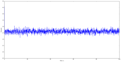
The energy, pressure and temperature plots vs time for the 0.001 time-step are shown in Figures 5, 6 and 7. All the plots tend to an average value, showing that the simulation is reaching equilibrium.

Figure 5. Energy vs time using a 0.001s time-step	Figure 6. Pressure vs time using a 0.001s time-step
Figure 7. Temperature vs time using a 0.001s time-step

Figure 5 shows the energy vs time for a time step of 0.001. It is obvious that this simulation reaches equilibrium as the graph tends to an average energy, after approximately 0.35s. Figure 8 shows the energy vs time for several time-steps all on one graph. The shorter the time-step, the better the simulation as shown by the smaller fluctuations in the graph once equilibrium has been reached. However, this requires more simulation steps for the same time period, thus requiring many more calculations. The 0.0025s time-step is the largest that tends to an average value similar to 0.001s and thus will be appropriate to use in further calculations to minimise time. The worst time step that could be taken out of those shown would be the 0.01s time-step, as the model doesn't tend to a value and demonstrating that it hasn't been able to reach equilibrium.

Figure 8. Energy vs time for multiple time steps

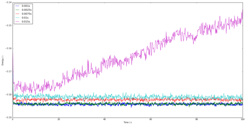
JC: Good choice of timestep, the average total energy should not depend on the timestep so 0.0075 and 0.01 are not suitable.

Running simulations under specific conditions

According to the equipartition theorem, each degree of freedom in a system at equilibrium with have $\frac{1}{2}{k}_{B}T$ energy. Considering our system with $N$ atoms and 3 degrees of freedom, the kinetic energy of the system is shown in equation 9.

$$\begin{gathered} E_k=\frac{3}{2}N{k}_{B}T=\frac{1}{2}\sum _i{m}_i{v}_i^2 \\ (9) \end{gathered}$$

However, the instantaneous temperature, T, fluctuates. We have a target temperature of $\mathfrak{𝔗}$, and to achieve this, we multiply each atoms velocity by a constant, $\gamma$, in order to ensure the kinetic energy of the system isn't too high or too low. This gives equation 10.

$$\begin{gathered} \frac{1}{2}\sum _i{m}_i{\left(\gamma v_i\right)}^2=\frac{3}{2}N{k}_B\mathfrak{𝔗} \\ (10) \end{gathered}$$

Which can be rewritten as:

$$\begin{gathered} \frac{1}{2}\sum _i{m}_i{\left(v_i\right)}^2=\frac{3}{2}N{k}_B\frac{\mathfrak{𝔗}}{{\gamma }^2} \\ (11) \end{gathered}$$

Combining equations (9) and (11):

$T=\frac{\mathfrak{𝔗}}{{\gamma }^2}$ $\gamma =\sqrt{\frac{\mathfrak{𝔗}}{T}}$

JC: Good.

The input file contains many over instructions. The following can be broken down to examine how the averages are being recorded:

fix aves all ave/time 100 1000 100000 v_dens v_temp v_press v_dens2 v_temp2 v_press2

100 (Nevery): The average is taken from points that are Nevery time-steps apart

1000 (Nrepeat): The average is taken over Nrepeat data points preceding the required averaged time-step, i.e. 1000.

10000 (Nfreq): The final average quantities in the data file occurs on time-steps that are multiples of Nfreq.

JC: Correct.

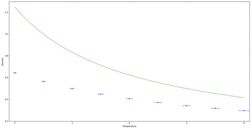
Graphs of density vs temperature for a pressure of 2.5 and 3.0 are shown in figures 9 and 10 respectively. Both graphs originally have a large difference between the computer modelled density and the density calculated using van der Waals equation. This suggests that the van der Waals approximation is in fact too simple at low temperatures, as it assumes the gas behaves as an ideal gas, with no intermolecular interactions. In fact, at the lower temperatures, the gas molecules are close enough for attractive intermolecular interactions to be significant. This makes the gas denser than predicted as an ideal gas. However, as the temperature increases, the gas has more kinetic energy allowing the atoms to overcome the attractive forces and disperse more, meaning the intermolecular interactions become weaker. Thus the ideal gas and simulated densities have less of a difference at higher temperatures. This effect is greater at a higher pressure, as the molecules are pushed together more and so have greater intermolecular interactions.

JC: Is this what your graphs show? The simulations are less dense than the ideal gas, not more dense, which suggests that the lack of repulsive interactions in the ideal gas is the most significant factor. The ideal gas is a good approximation to a dilute (high temperature, low pressure) gas. Plot all results on the same graph to see the trend with pressure more clearly.

Figure 9. Density vs Temperature for Pressure = 2.5

Figure 10. Density vs Temperature for Pressure = 3.0

Calculating heat capacities using statistical physics

It is possible to investigate the heat capacity of a system by considering the fluctuations in energy, using equation 12.

$$\begin{gathered} C_V=\frac{\partial E}{\partial T}=\frac{\mathrm{V}\mathrm{a}\mathrm{r}\left[E\right]}{k_B{T}^2}=N^2\frac{⟨E^2⟩-{⟨E⟩}^2}{k_B{T}^2} \\ (12) \end{gathered}$$

Figure 11 shows the heat capacity per unit cell against the temperature for the system at two different densities. The heat capacity of a system depends on the ability to promote molecules into higher energy levels at the cost of thermal energy, thus absorbing this thermal energy without increase the temperature of the system. Therefore, the more accessible rotational and vibrational energy states in the system available for promotion, the higher heat capacity of the system. As the temperature increases, many of these states start to become thermally occupied, and further promotion begins to become less enthalpically favourable.

Increasing the density means that there are now more atoms in the system, as we have kept the volume constant. This opens up the possibility of more rotational and vibrational energy level promotions before the states get saturated. Thus, the heat capacity is higher across the graph for the greater density.

Figure 11. Heat Capacity per unit cell vs Temperature
Density = 0.2	Density = 0.8
-1.15267900x10-05 $x$ + 3.63101786x10-05	-1.35550105x10-05 $x$ + 5.10905370x1005
R2=0.92985	R2=0.93113

JC: Your simulations are of classical, spherical particles, so there are no rotational or vibrational energy levels. However, you have the right idea to relate the heat capacity to the availability of energy levels, in this case the density of states. The heat capacity increases with density because the amount of energy required to raise the temperature of the system is proportional to the number of atoms per unit volume.

The input script had to be edited to carry out these simulations. The input script used for a T* = 2.2 and $\rho$* = 0.2 is shown below.

### SPECIFY THE REQUIRED THERMODYNAMIC STATE ###
variable T equal 2.2
variable dens equal 0.2
variable timestep equal 0.0025

### DEFINE SIMULATION BOX GEOMETRY ###
lattice sc ${dens}
region box block 0 15 0 15 0 15
create_box 1 box
create_atoms 1 box

### DEFINE PHYSICAL PROPERTIES OF ATOMS ###
mass 1 1.0
pair_style lj/cut/opt 3.0
pair_coeff 1 1 1.0 1.0
neighbor 2.0 bin

### ASSIGN ATOMIC VELOCITIES ###
velocity all create ${T} 12345 dist gaussian rot yes mom yes

### SPECIFY ENSEMBLE ###
timestep ${timestep}
fix nve all nve

### THERMODYNAMIC OUTPUT CONTROL ###
thermo_style custom time etotal temp press
thermo 10

### RECORD TRAJECTORY ###
dump traj all custom 1000 output-1 id x y z

### SPECIFY TIMESTEP ###

### RUN SIMULATION TO MELT CRYSTAL ###
run 10000
unfix nve
reset_timestep 0

### BRING SYSTEM TO REQUIRED STATE ###
variable tdamp equal ${timestep}*100
fix nvt all nvt temp ${T} ${T} ${tdamp}
run 10000
reset_timestep 0
unfix nvt
fix nve all nve

### MEASURE SYSTEM STATE ###
thermo_style custom step etotal temp atoms vol
variable etotal equal etotal
variable etotal2 equal etotal*etotal
variable temp equal temp
variable temp2 equal temp*temp
variable atoms2 equal atoms*atoms
variable vol equal vol
fix aves all ave/time 100 1000 100000 v_etotal v_etotal2 v_temp
run 100000

variable aveetotal equal f_aves[1]
variable aveetotal2 equal f_aves[2]
variable avetemp equal f_aves[3]
variable avetemp2 equal f_aves[3]*f_aves[3]
variable heatcapvol equal ${atoms2}*(f_aves[2]-f_aves[1]*f_aves[1])/(${avetemp2}*${vol})


print "Averages"
print "--------"
print "Ave E: ${aveetotal}"
print "Ave E2: ${aveetotal2}"
print "Atoms: ${atoms2}"
print "Temp: ${avetemp}"
print "Heat Capcity/Vol: ${heatcapvol}"

Structural properties and the radial distribution function

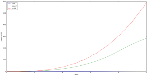
Figure 12 shows the Radial Distribution Function, or g(r), vs internuclear separation. The graph describes how the density of the system varies with the separation from the reference atom, or the likelihood of finding an atom at this distance from the reference atom. The integral of each phase is also shown in Figure 13, clearly showing that the density of a solid is much larger than the others, as more nuclei are found in the internuclear distance radius we have used.

Figure 12. RDF vs internuclear separation

Figure 13. RDF integral vs internuclear separation

The pressure and temperature values were adjusted to allow us to investigate 3 different phases, solid, liquid and gas, of the system using a phase diagram^[2]. All have a RDF of $\approx$ 0 at r = 0 to 1, as this is a region repulsive forces would be acting, and leading to a high potential. The first peak can be considered $r_{eq}$.

The easiest of the phases to analyse is the solid. As it is a solid, the atoms can generally be considered fixed, and it has the highest density of the 3 phases. In the short term separation, the graph displays sharp peaks. This demonstrates the high probability of the atom existing in a consistent lattice structure. There are four large peaks that drop in intensity but widen, showing the atoms to be located where expected but with small discrepancies in distance, broadening the peak. There are also smaller peaks, which represent defects in the crystal. The long range order is highly susceptible to defects, and that can be seen in the inconsistent peaks.

The liquid exhibits ever broadening peaks, until they are no longer visible. This shows that although there is still lattice structure like in the solid, it is much less rigid. The neighbouring atoms are more likely to be found over a range of distances from the reference atom, giving wide peaks.

The gas shows an even broader peak, demonstrating no real long range order. The system is fluid, and the least structured of all three.

Figure 14 shows a fcc lattice. If we consider the light blue atom to be the reference atom, the first three peaks at r = 0.975, 1.425 and 1.725 correspond to the green atoms, the dark blue atoms and the yellow atoms respectively. The lattice spacing corresponds to the distance between the reference atom and the dark blue atoms, and is therefore 1.425. The reference atom is coordinated to 12 green atoms, 6 dark blue atoms and 24 yellow atoms.

Figure 14. A face centred cubic unit cell, with different colours corresponding to different internuclear separations from the light blue reference atom

The integral of the RDF also shows notable differences for each state. It is expected that the magnitude of the integral at any distance is ordered solid>liquid>gas. The is expected due to the greater density of a solid, thus containing far more atoms per unit separation.

JC: The inconsistent peaks in the solid rdf are not due to defects, they are what you expect from an fcc lattice when you look at atoms separated by large distances. The broadening of the peaks is due to atoms vibrating around their lattice sites. The liquid has short range order, but no long range order. Good diagram of an fcc lattice, how did you calculate the number of nearest neighbours, did you check by looking at the integral of the rdf at short distances? What is the lattice parameter?

Dynamical properties and the diffusion coefficient

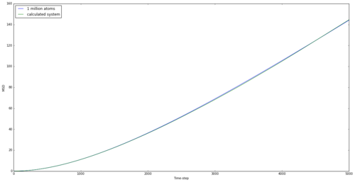
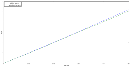
The mean squared displacement graphs for solid, liquid and gas are shown in Figures 15, 16 and 17 for both generated systems and the 1 million atom systems provided.

Figure 15. Vapour MSD	Figure 16. Liquid MSD
Figure 17. Solid MSD

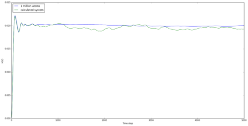The graphs are as expected. Atoms in solids are the most rigidly held and the large spike initially may be down to a small movement within the lattice. However, the move is below the lattice spacing and the atom doesn't move any further than this for the entire simulation, showing a rigid structure. The liquid shows a maximum displacement of just over 5, which shows that the atom is no longer rigid and can flow through the system. However the largest MSD is found with the gas, as expected. Being the least intermolecularly bonded system allows atoms to almost freely diffuse through space, and this is shown in the graph and by the highest diffusion coefficient. The simulations using 1 million atoms are seen to be smoother, suggesting a more realistic system, as this is considering a larger system from which to take averages.

The diffusion coefficient is given in equation 13.

$$\begin{gathered} D=\frac{1}{6}\frac{\partial ⟨r^2\left(t\right)⟩}{\partial t} \\ (13) \end{gathered}$$

This can therefore be calculated using the gradient of the MSD vs time graph, considering that each time-step represents 0.002s. The diffusion coefficients are shown in Table 3.

Table 3. Equations and coefficient of regressions used to calculate the diffusion coefficient, alongside the diffusion coefficient.

	Diffusion coefficient
	Simulation	1 million atoms
Solid	5.8333333x10-7	4.1666667x10-6
Liquid	8.3333333x10-2	8.3333333x10-2
Gas	2.7000000	2.5416667

JC: Plot the lines of best fit used to calculate D on the graphs. Did you fit a straight line to all of the data or just the linear part? Why does the gas phase MSD graph begin as a curved line (ballistic motion)?

The diffusion coefficient can also be calculated using the velocity autocorrelation function, shown as equation 14.

$$\begin{gathered} C\left(\tau \right)=\frac{\underset{-\mathrm{\infty }}{\overset{\mathrm{\infty }}{\int }}v\left(t\right)v(t+\tau )dt}{\underset{-\mathrm{\infty }}{\overset{\mathrm{\infty }}{\int }}{v}^2\left(t\right)dt} \\ (14) \end{gathered}$$

From the 1D harmonic oscillator, we know: $x(t)=A\cos (\omega t+\varphi )$, therefore $v(t)=\frac{\delta x(t)}{\delta t}=-A\omega \sin (\omega t+\varphi )$. This can be combined with equation 13 as follows:

$C\left(\tau \right)=\frac{\underset{-\mathrm{\infty }}{\overset{\mathrm{\infty }}{\int }}(-A\omega )\sin (\omega t+\varphi )(-A\omega )\sin (\omega (t+\tau )+\varphi )\mathrm{d}t}{\underset{-\mathrm{\infty }}{\overset{\mathrm{\infty }}{\int }}((-A\omega )\sin (\omega t+\varphi ){)}^2\left(t\right)\mathrm{d}t}$ $C(\tau )=\frac{\underset{-\mathrm{\infty }}{\overset{\mathrm{\infty }}{\int }}\sin (\omega t+\varphi )\sin (\omega t+\omega \tau +\varphi )dt}{\underset{-\mathrm{\infty }}{\overset{\mathrm{\infty }}{\int }}{\sin }^2(\omega t+\varphi )dt}$ $C(\tau )=\frac{\underset{-\mathrm{\infty }}{\overset{\mathrm{\infty }}{\int }}\sin (\omega t+\varphi )(\sin (\omega t+\varphi )\cos (\omega t)+\cos (\omega t+\varphi )\sin (\omega t)))dt}{\underset{-\mathrm{\infty }}{\overset{\mathrm{\infty }}{\int }}{\sin }^2(\omega t+\varphi )dt}$ $C(\tau )=cos(\omega t)\frac{\underset{-\mathrm{\infty }}{\overset{\mathrm{\infty }}{\int }}(si{n}^2(\omega t+\varphi ))dt}{\underset{-\mathrm{\infty }}{\overset{\mathrm{\infty }}{\int }}si{n}^2(\omega t+\varphi )dt}+\sin (\omega t)\frac{\underset{-\mathrm{\infty }}{\overset{\mathrm{\infty }}{\int }}(sin(\omega t+\varphi )cos(\omega t+\varphi ))dt}{\underset{-\mathrm{\infty }}{\overset{\mathrm{\infty }}{\int }}(si{n}^2(\omega t+\varphi ))dt}$

In the first term, $\underset{-\mathrm{\infty }}{\overset{\mathrm{\infty }}{\int }}(si{n}^2(\omega t+\varphi ))dt$ cancels.

$C(\tau )=cos(\omega t)+sin(\omega t)\frac{\underset{-\mathrm{\infty }}{\overset{\mathrm{\infty }}{\int }}(sin(\omega t+\varphi )cos(\omega t+\varphi ))dt}{\underset{-\mathrm{\infty }}{\overset{\mathrm{\infty }}{\int }}(si{n}^2(\omega t+\varphi ))dt}$

In the denominated in the fraction in the second term, we have an odd function, squared, giving an even function and a non-zero integral. However, the numerator contains an odd function multiplied by an even function, giving an odd function. This will have an integral of zero between $-\mathrm{\infty }$ and $+\mathrm{\infty }$, meaning the whole term is equal to zero. Therefore:

$C(\tau )=cos(\omega t)$

JC: Good.

Figure 18 is a plot of the VACFs for both the liquid and the solid with a harmonic oscillator. The obvious observation is that the harmonic oscillator is not a good representation of either system, as it demonstrates a conservation of kinetic energy that is not visible with the solid or liquid states. The starting system only contains potential energy, depicted when the system is randomly generated, but this order is lost with time, and the velocities of atoms become uncorrelated to their starting value. The result is both systems have tend to a $C(\tau )$ of 0.

The minima in these graphs represent a negative velocity compared to the starting velocity, or the return of the reference atom towards it's starting position. The solid has more of a rigid structure around it, and thus will hit barriers when travelling in one direction. It will rebound and head towards its original position and will continue to do this, thus the oscillations around 0. The liquid, however, is able to travel in one direction for much longer, simply losing kinetic energy through collisions until it's velocity is no longer connected with it's original value.

Figure 18. VACF vs time step

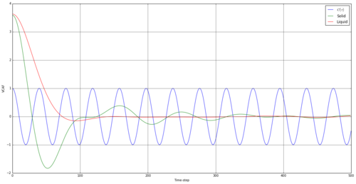
JC: Collisions between particles randomise particle velocities and cause the VACF to decorrelate, there are no collisions in the harmonic oscillator simulation so its VACF never decays to zero. It is not about conservation of kinetic energy.

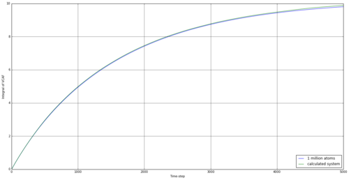
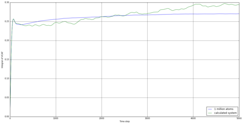
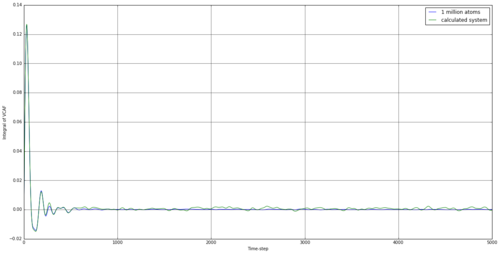
By taking the integral of the VACF data, we can establish how far the particle has indeed diffused. The simulated data was integrated using the trapezium rule, as well as the provided data for 1 million atoms. From this, we can use equation 15 to establish the diffusion coefficient. The results are shown in table 4.

$$\begin{gathered} D=\frac{1}{3}\underset{0}{\overset{\mathrm{\infty }}{\int }}\mathrm{d}\tau ⟨\mathbf{v}\left(0\right)\cdot \mathbf{v}\left(\tau \right)⟩ \\ (15) \end{gathered}$$

Figure 19. Vapour MSD	Figure 20. Liquid MSD
Figure 21. Solid MSD

Table 4. The diffusion coefficients calculated using the Velocity Autocorrelation Function for each phase.

	Diffusion coefficient
	Simulation	1 million atoms
Solid	-1.8453896x10-4	4.5587537x10-5
Liquid	9.7905916x10-2	9.0089602x10-2
Gas	3.2944994	3.2683770

The running integrals here are rather interesting. For the solid, there involves a large increase initially, but this is reversed quickly, and the integral fluctuates around 0 after less than 500 time steps. This would suggest the initial movement to be something similar to a vibration, with the reference atom transferring it's initial kinetic energy to other atoms and rebounding after it's initial movement. Overall, the simulation for a solid provided a negative diffusion coefficient, which was surprising but understandable, as the reference atom was making small vibrational movements at this time and could well be in the negative vector direction at the end of the simulation. The liquid simulation shows a large degree of diffusion initially, but this falls away towards the end of the simulation. This suggests that the rate of diffusion slows for a liquid over time. This effect is also observed in the vapour stage but the initial diffusion is much higher.

The resulting diffusion coefficients are similar for the 1 million atoms and our smaller simulation, apart from for the solid, suggesting our simulation is well representative of the larger system. The values are also of reasonable comparison to the values from the MSD method we investigated earlier, suggesting both can be used to back up the other.

One source of error in these calculation are using the trapezoid method for calculating the integral. We are limited to the size of the time-step in the original simulations, as this is the base of each individual trapezoid. Although it would require a longer computational time, a smaller time step would reduce any errors associated with this.

JC: The diffusion constant is only equal to the value of the integral when it has plateaued, you cannot say whether the rate of diffusion changes over time from these graphs. Since the simulations should be at equilibrium the diffusion coefficient should be constant too. The diffusion coefficient cannot be negative theoretically, the solid diffusion coefficient is effectively zero.

Conclusion

The importance of a small time step was established early in the experiment, as this meant that there were not large jumps between snapshots in which we were unaware of the interactions between atoms. However, it was clear that a compromise must be made between accuracy and computational time, as a smaller time step meant more calculations were required per run. The Lennard-Jones interaction model was used, and it was found that we could discard interactions above a certain internuclear distance, as this would again reduce the required calculations. We delved into the LAMMPS input script, allowing us to edit it to investigate different ensembles.

Plots of density vs temperature were made, demonstrating how the van der Waal's model is a poor approximation at low temperature due to intermolecular forces. This error was found to also be larger for greater pressures. The heat capacity per unit cell was also plotted against temperature, and this was found to decrease with an increase in temperature as it gets thermodynamically less favourable to undergo further promotions in energy states. The heat capacity was greater for higher densities, due to more atoms being available for excitation. The RDFs were plotted for three different phases, and showed the solid phase to exhibit much stronger structural order than the other two, as expected. The three phases could be easily distinguished using this computational method. The diffusion coefficient was calculated using two different methods. Although there were slight discrepancies, the values returned were similar using both methods.

References

[1] Ercolessi, F. (1997). The Verlet algorithm. [online] Available at: http://www.citethisforme.com/guides/harvard/how-to-cite-a-website [Accessed 06/03/17].

[2] Hansen, J and Verlet, L. (1969). Phase Transitions of the Lennard-Jones System. Phys. Rev. 184, 151.