Talk:Mod:EZPython
JC: General comments: A few small mistakes, but on the whole a good report. You have demonstrated that you have a good understanding of the Ising model and of the steps of this practical, well done.
Programming for simple simulaitons - CMP
Introduction to Ising model
Task 1: Lowest energy, multiplicity and entropy.
Given that , energy will be at its minimum when all the spins are parallel, ie. have the same sign.
When boundary conditions are applied in a 1D system with total number of spins ; each spin has 2 neighbouring spins. In a corresponding 2D system, each spin has 4 neighbouring spins and for a corresponding 3D system, 6 neighbours. This gives: It is clear that a general trend can be seen where constant in the equation is simply a dimension of the given system. We can therefore rewrite the equation as
Multiplicity can be found using where is the total number of spins and is the number of spins in the state . Since the number of states in this system is 1 multiplicity .
Entropy is given my expression Therefore for a system in its lowest energy state, entropy . This is the value we would expect since any system in its lowest energy state will be fully ordered and hence will have minimum entropy. W
JC: In the ground state the spins are all parallel, but they can be pointing up or down, so the multiplicity of this state is actually 2 and the entropy is 9.57e-24.
Task 2: Energy of a system with one spin up
Using the formula derived in the previous task, minimum energy of the system is . When one spin is changed in a 3D system, 6 neighbouring spins are affected by the change and 993 remain unaffected. Therefore when calculating the total energy of the system with one spin flipped, we need to consider the total energy of 993 spins; energy of one flipped spin and the sum of energies of 6 neighbouring atoms. Total energy is therefore . Hence the change in energy is simply .
JC: This is correct, well done.
As preciously stated entropy of a system in lowest energy state is . In order to find the entropy of a system with one spin flipped we need to find multiplicity of such system. New multiplicity of the state with one spin flipped will be since it can have 2 different orientations in any of the 1000 different lattice points. Hence
JC: Multiplicity of state with single spin flipped is 2000, but the difference in entropy should be .
Task 3: Magnetisation
Magnetisation of a system is given by the equation where is the spin.
Lattice system with 3 spins pointed up and 2 spins down has magnetisation .
Lattice system with 13 spins pointing up and 12 spins down has magnetisation .
At an absolute zero, , Isling Lattice is a fully ordered system in its lowest energy state where all the spins are parallel and of the same orientation. We can therefore calculate magnetisation .
JC: Correct, since magnetisation in ground state can be +1000 or -1000, the multiplicity of the ground state must be 2.
Calculating the energy and magnetisation
Task 1: Calculating the total Energy and Magnetisation
Following code loops over each row and column of a random Ising Lattice previously created and calculates its total Energy, and Magnetisation, .
import numpy as np

class IsingLattice:
    E = 0.0
    E2 = 0.0
    M = 0.0
    M2 = 0.0

    n_cycles = 0

    def __init__(self, n_rows, n_cols):
        self.n_rows = n_rows
        self.n_cols = n_cols
        self.lattice = np.random.choice([-1,1], size=(n_rows, n_cols))
    def energy(self):
        energy = 0.0
        #following two lines loop over each row and column in the system
        for i in range (self.n_rows):
            for j in range (self.n_cols):
                system = self.lattice[i][j]
                #following code makes sure periodic boundary condition is held
                #Making sure that top row energies are calculated separetly to the rest following boundary condition
                if i > 0:
                    energy += -0.5*(self.lattice[i-1,j]*system)
                else:
                    energy += -0.5*(self.lattice[-1,j]*system)
                #Making sure that first column energies are calculated separatley to the rest following periodic boundary condition
                if j > 0:
                    energy += -0.5*(self.lattice[i,j-1]*system)
                else:
                    energy += -0.5*(self.lattice[i,-1]*system)
                #Making sure that bottom row energies are calculated separatley to the rest following periodic boundary condition
                if i < self.n_cols-1:
                    energy += -0.5*(self.lattice[i+1, j]*system)
                else:
                    energy += -0.5*(self.lattice[0,j]*system)
                #Making sure that last column energies are calculated separatley to the rest following periodic boundary condition
                if j < self.n_rows-1:
                    energy += -0.5*(self.lattice[i,j+1]*system)
                else:
                    energy += -0.5*(self.lattice[i,0]*system)
        return energy

    def magnetisation(self):
        magnetisation = 0.0
        #following two lines loop over each row and column in the system
        for i in range (self.n_rows):
            for j in range (self.n_cols):
                magnetisation += self.lattice[i][j]
        return magnetisation
Task 2: Checking the code
Code presented above was run using the ILcheck.py script provided and image presented in Figure 1. was produced.

Figure 1 shows an Ising Lattice
with different spin configurations. Lattice on the left is in its lowest energy state. Middle lattice has a random spin configuration with random Energy and final lattice is in the highest energy state. In lowest energy configuration all the spins are aligned and of the same orientation. As predicted by the energy formula previously discussed
where J is assumed to be 1,
. Magnetisation is also matches the expected
. Highest energy state is produced by alternating spins (+1/-1) thereby cancelling out the total magnetisation,
.
JC: Your code is correct and very well commented and explained. You actually don't even need the if statement for i>0 or j>0, but this is a very minor point.
Introduction to Monte Carlo simulation
Task 1: For a lattice with 100 spins and 2 ways of arranging each spin there are ways of arranging the system. If we assume that configurations can be analysed each second it would take s which is an equivalent of years to complete the simulation. This is an unreasonable timescale and therefore some
code adjustments need to be implemented in order to increase the efficiency of our calculations.
JC: Your answer is correct in seconds, but the conversion to years is incorrect, should be about 4e13 years.
Task 2: Following code is of a Monte Carlo function which returns energies and magnetisations of a given lattice.
def montecarlostep(self, T):
        energy = self.energy()

        #the following two lines will select the coordinates of the random spin for you
        random_i = np.random.choice(range(0, self.n_rows))
        random_j = np.random.choice(range(0, self.n_cols))
        #defiing a new nadom lattice
        self.lattice[random_i][random_j] = - self.lattice[random_i][random_j]
        #defining a function that will flip the random latice
        #calculating energy for the flipped lattice
        flip_energy = self.energy()
        #magnetisation value is calculated using magnitisation function
        flip_magnetisation = self.magnetisation()
        #calculating the energy difference between flipped spin lattice and the original lattice
        energy_change = flip_energy - energy
        # if the flip reduced energy we set new energy value to be original energy
        if energy_change < 0:
                energy = energy_change
        # if energy goes up we chose a random number in [0,1) interval to decide if we reset energy or leave it unchanged
        elif energy_change > 0:
        #the following line chooses a random number in the rang e[0,1)
            random_number = np.random.random()
            #if random number is smaller than specific value, we set new energy value to be original energy
            if random_number <= np.exp(-(energy_change)/(T)):
                energy = energy_change
            #otherwise we flip the lattice again to bring it back to the original
            else:
                self.lattice[random_i][random_j] = - self.lattice[random_i][random_j]

        #all new energies and magnetisations produced are appended to the original object to get the running total
        self.E += energy
        self.M += magnetisation_1
        #new energy and magnetisation squared values are calculated and appended to the original object to get the running total
        self.E2 += energy*energy
        self.M2 += magnetisation_1*magnetisation_1
        #number of itterations carried out in total is calculated by adding 1 to the total with each new loop
        self.n_cycles += 1

        return energy, flip_magnetisation


    def statistics(self):
        averageE = self.E/self.n_cycles
        averageE2 = self.E2/self.n_cycles
        averageM = self.M/self.n_cycles
        averageM2 = self.M2/self.n_cycles
        return averageE, averageE2, averageM, averageM2
JC: In your Monte Carlo code when you accept the new configuration you should make energy = flip_energy not energy_change. You also don't define magnetisation_1 which should mean that your code exits with an error, so I think this must be an older version of your code.
Task 3:
Currie Temperature is a critical temperature above which our lattice is paramagnetic with all of its spins randomly orientated. At T < T_c system undergoes spontaneous symmetry breaking and rearranges to a ferromagnetic lattice with all of the spins aligned and pointing in the same direction. Ferromagnetic system has a larger magnetic susceptibility than the paramagnetic system and is in the lower energy state. It is therefore expected that below T_c system would undergoes spontaneous magnetisation to reduce its energy.
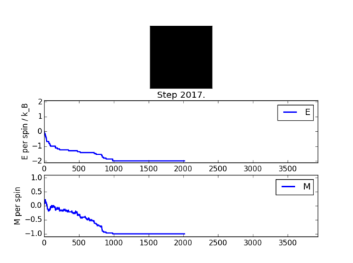
ILanim.py script was run to check that Monte Carlo function stated above carries out the correct simulation. Figure 2 shows that the simulation indeed works and that the system reaches equilibrium at around 1000 steps. Spontaneous magnetisation occurred during the simulation, suggesting that temperature used was below the T_c. Table 1. shows the
results obtained using the statistics function in the Monte Carlo code.
| Table 1. | |
|---|---|
| E | -1.67 |
| E2 | 2.984 |
| M | -0.707 |
| M | 0.638 |
Accelerating the code
ILtimetrial.py script was run with the original IsingLattice.py (energy and magnetisation code previously shown) to determine the time is takes for the code to finish its calculation. Code was then accelerated substituting loops in the original code with new Python functions such as np.sum, np.multyply and np.roll. New accelerated code is presented below.
def energy(self):
        total_energy = 0.0
       #np.roll function makes sure the boundary conditions are kept as it rolls the lattice array 1 along in both rows(0)                and columns(1) with each iteration
       #factor of a half is no longer needed since rows and columns are now only rolled in one direction producing a single value
       #np.muliply multiplies two neighbouring spins by multiplying the lattice with its rolled array
       #np.sum sums all the products of the neighbouring spins in both x = rows and y = cols direction
       #total energy is the sum of x and y energies
        total_energy = np.sum(-np.multiply(self.lattice, np.roll(self.lattice,1,0)))+np.sum(-np.multiply(self.lattice, np.roll(self.lattice,1,1)))
        return total_energy
def magnetisation(self):
        magnetisaton = 0.0
        #since magnetisation is simply the sum of all lattice points, np.sum function is used to add all the values up insead of appending each in a loop
        magnetisation = np.sum(self.lattice)
        return magnetisation
The accelerated version of the code was then used to run the Monte Carlo simulation and time elapsed was again checked using the ILtimetrial.py script. Table 2. shows the time take to run the simulation with the original code and the new accelerated version. Standard error was calculated for 5 repeats. It is clear that the new version of the code is a much more efficient and is preferred for out simulation.
| Table 2. | ||||||
|---|---|---|---|---|---|---|
| Code type | Time (s) | Standard Error | ||||
| Original | 155.8406 | 155.5866 | 145.7004 | 161.1409 | 153.5225 | 2.503685 |
| Accelerated | 1.2489 | 1.2473 | 1.2086 | 1.1946 | 1.2779 | 0.0150 |
JC: The numpy functions are correctly used to accelerate the code. You should calculate an average time for the original and accelerated code. Try to make sure that the comments don't run off the edge of the wiki page.
The effect of temperature
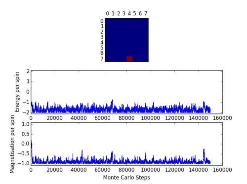
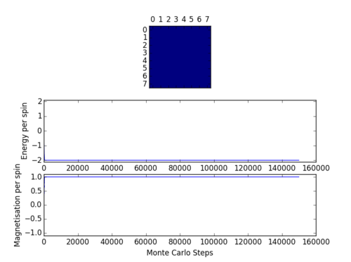
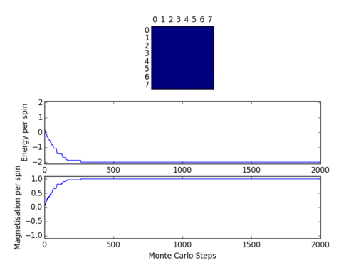
Effect of temperature and lattice size on the speed of the equilibration of the system was analysed. Table 3 shows the effect of temperature change on an 8x8 lattice. Temperatures of above and below 1 were used to see the effect relative to the system at T=1. It was found that system equilibrates at temperatures below 1 but it is not possible to establish the exact time when the equilibrium is reached as it happens very early on in the simulation with 150000 steps. Lower run times were used to establish approximate time at which equilibrium is reached. It was clear that it took less time to reach equilibrium at lower temperatures.
A much smaller 3x3 lattice was analysed. It was assumed that a smaller lattice will require much less time to equilibrate and therefore run time was set to 150 Monte Carlo steps. As expected system did not equilibrate above T=1 and equilibrated very quickly at T=1.
JC: What number of Monte Carlo steps did you decide to use as a cut off to ensure that the simulation reached equilibrium before you started to collect data? You should have given the updated code for the statistics() function to show how you included the cut off.

JC: Can you comment on this graph and what it shows.
The effect of system size
The effect of system size was studied running the above code for systems of different size. Run time and time after which average values are calculated was chosen separate for each system according to results previously obtained to save time and improve accuracy. Results are summarised in Table 6.
| Table 6. Effect of system size | |||
|---|---|---|---|
| Size | Run time | Average after | Graph |
| 2x2 | 1000 | 50 | 
|
| 4x4 | 2000 | 100 | 
|
| 8x8 | 10000 | 1000 | 
|
| 16x16 | 15000 | 10000 | 
|
| 32x32 | 150000 | 120000 | 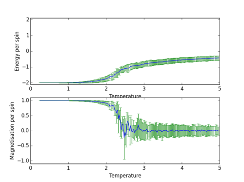
|
All the results where then plotted on one graph to have a clear comparison - Figure 4. Due to very frequent sampling, graph of all the systems looked extremely busy, it was therefore decided to plot without the error bars. Code used is presented below (error bars and error calculations are hash tagged since they were not used):
from matplotlib import pylab as pl
import numpy as np
#unpacking text files with data
temps2, energies2, energysq2, magnetisations2, magnetisationsq2 = np.loadtxt("2x2.dat", unpack=True)
temps4, energies4, energysq4, magnetisations4, magnetisationsq4 = np.loadtxt("4x4.dat", unpack=True)
temps8, energies8, energysq8, magnetisations8, magnetisationsq8 = np.loadtxt("8x8.dat", unpack=True)
temps16, energies16, energysq16, magnetisations16, magnetisationsq16 = np.loadtxt("16x16.dat", unpack=True)
temps32, energies32, energysq32, magnetisations32, magnetisationsq32= np.loadtxt("32x32".dat, unpack=True)

#number of cycles take to obtain averages and spins for each system need to be stated for error calculations and graph ploting
n_average2 = 950
spins2 = 4
n_average4 = 1900
spins4 = 16
n_average8 = 3000
spins8 = 64
n_average16 = 5000
spins16 = 256
n_average32 = 30000
spins32 = 1024

#calculating errors for each system if error bars need plotting
#errorE2 = np.sqrt(np.divide((energysq2- np.multiply(energies2,energies2)), (n_average2)))
#errorM2 = np.sqrt(np.divide((magnetisationsq2- np.multiply(magnetisations2,magnetisations2)), (n_average2)))
#errorE4 = np.sqrt(np.divide((energysq4- np.multiply(energies4,energies4)), (n_average4)))
#errorM4 = np.sqrt(np.divide((magnetisationsq4- np.multiply(magnetisations4,magnetisations4)), (n_average4)))
#errorE8 = np.sqrt(np.divide((energysq8- np.multiply(energies8,energies8)), (n_average8)))
#errorM8 = np.sqrt(np.divide((magnetisationsq8- np.multiply(magnetisations8,magnetisations8)), (n_average8)))
#errorE16 = np.sqrt(np.divide((energysq16- np.multiply(energies16,energies16)), (n_average16)))
#errorM16 = np.sqrt(np.divide((magnetisationsq16- np.multiply(magnetisations16,magnetisations16)), (n_average16)))
#errorE32 = np.sqrt(np.divide((energysq32- np.multiply(energies32,energies32)), (n_average32)))
#errorM32 = np.sqrt(np.divide((magnetisationsq32- np.multiply(magnetisations32,magnetisations32)), (n_average32)))

#configuring the graphs, ie labels and axis range
fig = pl.figure()
enerax = fig.add_subplot(2,1,1)
enerax.set_ylabel("Energy per spin")
enerax.set_xlabel("Temperature")
enerax.set_ylim([-2.1, 2.1])

magax = fig.add_subplot(2,1,2)
magax.set_ylabel("Magnetisation per spin")
magax.set_xlabel("Temperature")
magax.set_ylim([-1.1, 1.1])

#Plotting each energy graph with corresponding error bars if wanted
enerax.plot(temps2, np.array(energies2)/spins2, label="2x2")
#enerax.errorbar(temps2, np.array(energies2)/spins2,yerr=errorE2, linestyle="None")
enerax.plot(temps4, np.array(energies4)/spins4, label="4x4")
#enerax.errorbar(temps4, np.array(energies4)/spins4,yerr=errorE4,linestyle="None")
enerax.plot(temps8, np.array(energies8)/spins8, label="8x8")
#enerax.errorbar(temps8, np.array(energies8)/spins8,yerr=errorE8,linestyle="None")
enerax.plot(temps16, np.array(energies16)/spins16, label="16x16")
#enerax.errorbar(temps16, np.array(energies16)/spins16,yerr=errorE16,linestyle="None")
enerax.plot(temps32, np.array(energies32)/spins32, label="32x32")
#enerax.errorbar(temps32, np.array(energies32)/spins32,yerr=errorE32,linestyle="None")
enerax.legend(loc="upper right", fontsize = "x-small")

#plotting each magnetisation with corresponding error bars
magax.plot(temps2, np.array(magnetisations2)/spins2,label="2x2")
#magax.errorbar(temps2, np.array(magnetisations2)/spins2,yerr=errorM2,linestyle="None")
magax.plot(temps4, np.array(magnetisations4)/spins4, label="4x4")
#magax.errorbar(temps4, np.array(magnetisations4)/spins4,yerr=errorM4,linestyle="None")
magax.plot(temps8, np.array(magnetisations8)/spins8, label="8x8")
#magax.errorbar(temps8, np.array(magnetisations8)/spins8,yerr=errorM8,linestyle="None")
magax.plot(temps16, np.array(magnetisations16)/spins16, label="16x16")
#magax.errorbar(temps16, np.array(magnetisations16)/spins16,yerr=errorM16,linestyle="None")
magax.plot(temps32, np.array(magnetisations32)/spins32, label="32x32")
#magax.errorbar(temps32, np.array(magnetisations32)/spins32,yerr=errorM32,linestyle="None")
magax.legend(loc="upper right", fontsize = "x-small")

pl.show()

From Figure 4 we can see that 8x8 system matches energies and magnetisations of larger systems with an insignificantly larger error. It can therefore be concluded that 8x8 lattice is large enough to capture long range fluctuations and small enough to carry out simulations fast and efficient.
JC: Good use of loadtxt function in the plot code and identified 8x8 system as smallest system able to capture fluctuations.
Determining the heat capacity
Heat capacity can be dirived from .
Average energy is given by , where partition function .
Hence
Where and
Therefore
JC: Good, clear derivation.
is easy to calculate using the values of average energies squared and average energies returned and stored in a data file using code from 'The effect of temperature' section for each analysed system. Since we now have all the data needed we can calculate heat capacity and plot it as a function of temperature. Figure 5 shows the resulting graph for all of the systems. Code used to do this calculation is presented below:
from matplotlib import pylab as pl
import numpy as np
#unpacking text files with data
temp2, energy2, energysq2 = np.loadtxt("2x2.dat", usecols=(0,1,2), unpack=True)
temp4, energy4, energysq4 = np.loadtxt("4x4.dat", usecols=(0,1,2), unpack=True)
temp8, energy8, energysq8 = np.loadtxt("8x8.dat", usecols=(0,1,2), unpack=True)
temp16, energy16, energysq16 = np.loadtxt("16x16.dat", usecols=(0,1,2), unpack=True)
temp32, energy32, energysq32 = np.loadtxt("32x32.dat", usecols=(0,1,2), unpack=True)

spins2 = 4
spins4 = 16
spins8 = 64
spins16 = 256
spins32 = 1024

#variance of energy was calulated for each system
#np.divide function was used divide varince of energy by temperature squared calculated using np.multiply
#those functions were used to manipulate arrays continuosly.
var2 = energysq2-np.multiply(energy2,energy2)
C_2 = np.divide(var2, (np.multiply(temp2,temp2)))
var4 = energysq4-np.multiply(energy4,energy4)
C_4 = np.divide(var4, (np.multiply(temp4,temp4)))
var8 = energysq8-np.multiply(energy8,energy8)
C_8 = np.divide(var8, (np.multiply(temp8,temp8)))
var16 = energysq16-np.multiply(energy16,energy16)
C_16 = np.divide(var16, (np.multiply(temp16,temp16)))
var32 = energysq32-np.multiply(energy32,energy32)
C_32 = np.divide(var32, (np.multiply(temp32,temp32)))

fig = pl.figure()
hcaxis = fig.add_subplot(2,1,1)
hcaxis.set_ylabel("Heat capacity")
hcaxis.set_xlabel("Temperature")
hcaxis.plot(temp2, np.array(C_2)/spins2, label = "2x2")
hcaxis.plot(temp4, np.array(C_4)/spins4, label = "4x4")
hcaxis.plot(temp8, np.array(C_8)/spins8, label = "8x8")
hcaxis.plot(temp16, np.array(C_16)/spins16, label = "16x16")
hcaxis.plot(temp32, np.array(C_32)/spins32, label = "32x32")
hcaxis.legend(loc="upper right", fontsize = "x-small")
pl.show()

With an increase in lattice size, heat capacity peak becomes sharper and heat capacity increases. Peak appears in the expected region for Currie temperature around 2-2.5 (temperature above which no spontaneous magnetisation occurred in our simulation in 'Effect of temperature' section). It is expected that when T = T_c a phase transition from ferromagnetic to paramagnetic spin state will occur. Heat capacity for an infinitly large system will be infinity at this phase transition as the change in the symmetry of our lattice system is discontinuous.
JC: Heat capacity calculated correctly in your code. You don't need to use the numpy functions multiply and divide here as you are working with floats, not arrays, so they won't speed up you code as they did in the energy() and magnetisation() functions.
Locating the Curie temperature
Data obtained from much longer simulations using C++ was compared to the data produced with Python code. All calculated values were plotted on the same graph against temperature to see how the data differs. Figure 6 shows such graph for the largest lattice of 32x32 since is produced least fluctuation and error in Python therefore was easier to compare. Code to plot such a comparison is presented below. Number 32 can be substituted for dimentions of another lattice to plot a new graph.
from matplotlib import pylab as pl

import numpy as np
#unpacking Python text files with data
temps2, energies2, energysq2, magnetisations2, magnetisationsq2 = np.loadtxt("2x2.dat", unpack=True)
temps4, energies4, energysq4, magnetisations4, magnetisationsq4 = np.loadtxt("4x4.dat", unpack=True)
temps8, energies8, energysq8, magnetisations8, magnetisationsq8 = np.loadtxt("8x8.dat", unpack=True)
temps16, energies16, energysq16, magnetisations16, magnetisationsq16 = np.loadtxt("16x16.dat", unpack=True)
temps32, energies32, energysq32, magnetisations32, magnetisationsq32= np.loadtxt("32x32.dat", unpack=True)
#unpacking C++ text files with data
temps2C, energies2C, energysq2C, magnetisations2C, magnetisationsq2C, hcC2 = np.loadtxt("2x2C.dat", unpack=True)
temps4C, energies4C, energysq4C, magnetisations4C, magnetisationsq4C, hcC4 = np.loadtxt("4x4C.dat", unpack=True)
temps8C, energies8C, energysq8C, magnetisations8C, magnetisationsq8C, hcC8 = np.loadtxt("8x8C.dat", unpack=True)
temps16C, energies16C, energysq16C, magnetisations16C, magnetisationsq16C, hcC16 = np.loadtxt("16x16C.dat", unpack=True)
temps32C, energies32C, energysq32C, magnetisations32C, magnetisationsq32C, hcC32 = np.loadtxt("32x32C.dat", unpack=True)

#spin values for python systems
spins2 = 4
spins4 = 16
spins8 = 64
spins16 = 256
spins32 = 1024

#configuring a plot with 5 graphs plotted simultaneously (first argument in add_subplot is 5)
fig = pl.figure()

enerax32 = fig.add_subplot(5,1,1)
enerax32.set_ylabel("Energy per spin", fontsize = "x-small")
enerax32.set_xlabel("Temperature", fontsize = "x-small")
enerax32.set_ylim([-2.1, 2.1])

enersqax32 = fig.add_subplot(5,1,2)
enersqax32.set_ylabel("E^2 per spin", fontsize = "x-small")
enersqax32.set_xlabel("Temperature", fontsize = "x-small")
enersqax32.set_ylim([0, 5])

magax32 = fig.add_subplot(5,1,3)
magax32.set_ylabel("Magnetisation per spin", fontsize = "x-small")
magax32.set_xlabel("Temperature", fontsize = "x-small")
magax32.set_ylim([-1.1, 1.1])

magsqax32 = fig.add_subplot(5,1,4)
magsqax32.set_ylabel("M^2 per spin", fontsize = "x-small")
magsqax32.set_xlabel("Temperature",fontsize = "x-small")
magsqax32.set_ylim([0, 2])

#finding heat capacity of python system
var32 = energysq32-np.multiply(energies32,energies32)
C_32 = np.divide(var32, (np.multiply(temps32,temps32)))

hcaxis32 = fig.add_subplot(5,1,5)
hcaxis32.set_ylabel("Heat capacity", fontsize = "x-small")
hcaxis32.set_xlabel("Temperature", fontsize = "xx-small")
hcaxis32.set_ylim([-1, 2])
#plotting both versions on one graph
enerax32.plot(temps32, np.array(energies32)/spins32, label="32x32")
enerax32.plot(temps32C, np.array(energies32C), label="32x32 C++")
enerax32.legend(loc="upper right", fontsize = "xx-small")

enersqax32.plot(temps32, np.array(energysq32)/spins32, label="32x32")
enersqax32.plot(temps32C, np.array(energies32C), label="32x32 C++")
enersqax32.legend(loc="upper right", fontsize = "xx-small")

magax32.plot(temps32, np.array(magnetisations32)/spins32, label="32x32")
magax32.plot(temps32C, np.array(magnetisations32C), label="32x32 C++")
magax32.legend(loc="upper right", fontsize = "xx-small")

magsqax32.plot(temps32, np.array(magnetisationsq32)/spins32, label="32x32")
magsqax32.plot(temps32C, np.array(magnetisationsq32C), label="32x32 C++")
magsqax32.legend(loc="upper right", fontsize = "xx-small")


hcaxis32.plot(temps32, np.array(C_32)/spins32, label = "32x32")
hcaxis32.plot(temps32C, np.array(hcC32), label = "32x32 C++")
hcaxis32.legend(loc="upper right", fontsize = "xx-small")


pl.show()
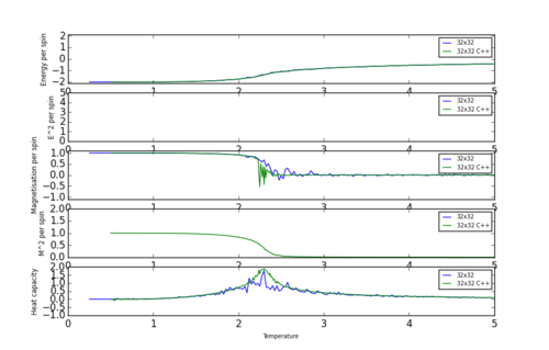
Figure 6 shows that data compares very well and that heat capacity peaks and phase transitions occur at the same temperature on both Python and C++. Python data does show slight discrepancy and not as smooth as C++ data for Magnetisation and Heat capacity calculations. This is due to C++ data being sampled more often and over a longer period of time resulting in greater number of data points, giving a more continuous and hence accurate plot.
JC: Why do the discrepancies occur around the Curie temperature?
Polynomial fitting:
Following code was used to fit a polynomial to the data:
from matplotlib import pylab as pl
import numpy as np
#first and last colums of dat file extracted
data = np.loadtxt("16x16C.dat", usecols=(0,5))
T = data[:,0] #get the first column
C = data[:,1] # get the second column

#For a 16x16 lattice a 100th degree polynomial is fitted for all temperatures and heat capacity values
fit = np.polyfit(T, C, 100)

#now we generate interpolated values of the fitted polynomial over the range of our function
T_min = np.min(T)
T_max = np.max(T)
T_range = np.linspace(T_min, T_max, 1000) #generate 1000 evenly spaced points between T_min and T_max
fitted_C_values = np.polyval(fit, T_range) #use the fit object to generate the corresponding values of C
#plot the graph and its polynomial fit
fig = pl.figure()
hcaxis = fig.add_subplot(1,1,1)
hcaxis.set_ylabel("Heat capacity", fontsize = "small")
hcaxis.set_xlabel("Temperature", fontsize = "small")
hcaxis.set_ylim([-1, 3])

hcaxis.plot(T, C, label = "Original")
hcaxis.plot(T_range, fitted_C_values, label = "Fitted")
hcaxis.legend(loc="upper right", fontsize = "small")

pl.show()
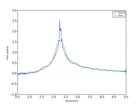
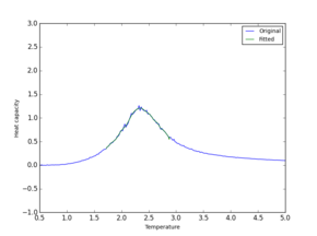
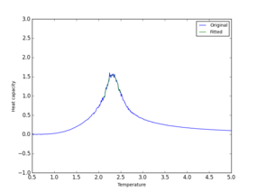
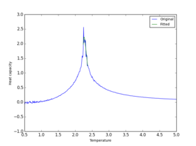
Polynomial fitting was simpler for smaller sysytems and worked well up to a 16x16 lattice. Larger systems require higher dergee of polynomial. It was found that polynomial can be fitted more efficiently and accuratly if a smaller range of T and C values are used. Code was adjusted to give a better fit:
from matplotlib import pylab as pl
import numpy as np

data = np.loadtxt("2x2C.dat", usecols = (0,5))
T = data[:,0]
C = data[:,1]

#choosing a minimum and maximum temperature for the polynomial
T_min = 2.1
T_max = 2.5
#make sure value is chosen from the range
selection = np.logical_and(T > T_min, T < T_max)
peak_T_values = T[selection]
peak_C_values = C[selection]
fit = np.polyfit(peak_T_values, peak_C_values, 100)
#generate 1000 evenly spaced points between the minimum and maximum T for the peak
T_range = np.linspace(np.min(peak_T_values), np.max(peak_T_values), 1000)
#fitting the heat capacity polyomial corresponding to the range of temperature values
fitted_C_values = np.polyval(fit, T_range)

fig = pl.figure()
hcaxis = fig.add_subplot(1,1,1)
hcaxis.set_ylabel("Heat capacity", fontsize = "small")
hcaxis.set_xlabel("Temperature", fontsize = "small")
hcaxis.set_ylim([-1, 3])

hcaxis.plot(T, C, label = "Original")
hcaxis.plot(T_range, fitted_C_values, label = "Fitted")
hcaxis.legend(loc="upper right", fontsize = "small")

pl.show()
JC: Code is well commented, shows that you have a good understanding of what polyval and polyfit do.
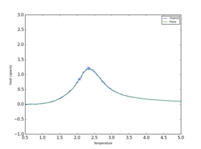
Two polynomial fits are compared in Table 7 It is clear that a much more accurate value for Currie temperature and Heat Capacity can now be found using the plot.
| Table 7. Polynomial fit | ||||
|---|---|---|---|---|
| System | 2x2 | 8x8 | 16x16 | 64x64 |
| Full range | 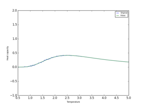
|
|

|
|
| Peak only | 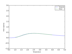
|
|
|
|
Finding the peak in C:
Maximum value for heat capacity and the corresponding temperature was found using np.max funtion on all the C++ data files provided. Table 8 summarises the findings for all of the systems.
Cmax = np.max(fitted_C_values)

Tmax = T_range[fitted_C_values == Cmax]

print(Tmax, Cmax)
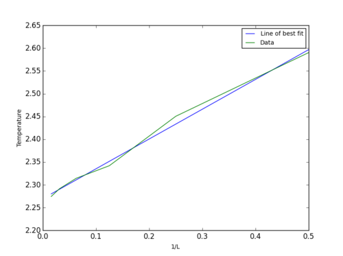
Temperatures obtained were then used to plot temperature against 1/(lattice legth) and hence using scaling relationship ( T_{C,L} = \frac{A}{L} + T_{C,\infty} ) obtain values for constants A and Curie temperature of an infinite lattice, y itercept - T_{C,\infty}. Data obtained was ploted using the code below:
JC: Use "math" formatting here.
from matplotlib import pylab as pl
import numpy as np
x = [1/2, 1/4, 1/8, 1/16, 1/32, 1/64]
y = [2.59037037, 2.45051051, 2.34198198, 2.31426426, 2.29144144,  2.27432432]

fit = np.polyfit(x, y, 1)
x_min = np.min(x)
x_max = np.max(x)
x_range = np.linspace(x_min, x_max, 1000) #generate 1000 evenly spaced points between T_min and T_max
fitted_x_values = np.polyval(fit, x_range)

fig = pl.figure()
xy = fig.add_subplot(1,1,1)
xy.set_ylabel("Temperature", fontsize = "small")
xy.set_xlabel("1/L", fontsize = "small")
xy.set_ylim([2.2, 2.65])
xy.plot(x_range, fitted_x_values, label = "Line of best fit")
xy.plot(x, y, label = "Data")
xy.legend(loc="upper right", fontsize = "small")
pl.show()
| Table 8. | ||
|---|---|---|
| Lattice size | Heat capacity | Temperature |
| 2x2 | 0.41761453108 | 2.59037037 |
| 4x4 | 0.81568383612 | 2.45051051 |
| 8x8 | 1.19921782038 | 2.34198198 |
| 16x16 | 1.5592144128 | 2.31426426 |
| 32x32 | 1.8570969502 | 2.29144144 |
| 64x64 | 2.1550995064 | 2.27432432 |
Figure 7 shows the graph obtained together with a line of best fit used to find the T_{C,\infty} = 2.27437. This obtained value agrees very well with an exact calculated value of 2.269 (H.A. Kramers and G.H. Wannier, Phys. Rev. 60, 252 (1941)). A small 1% error could be due to the calulated energy and magnetisation average values not being totally accurate. From C++ code provided below, it can be seen that average values were calculation after 100*(number of spins) Monte Carlo cycles. This means that for systems larger than 32x32, average value is being calculated before complete equilibration is reached (ie. 102000 when equilibration is reached at approximately 120000). This, together with a non-exact polynomial fit used to obtain peak values, results in an insignificant error demonstrated in our results.
JC: Fit looks good and good estimate of Curie temperature. Well done for looking into the C++ code to see how the simulations are set up as well.
IsingLattice il(L, L);
const int cutoff = 100*Nspins;
double E = 0.0;
double E2 = 0.0;
double M = 0.0;
double M2 = 0.0;
for (int i = 0; i < Nsteps*Nspins; ++i) {
   il.montecarlostep(T);
   if (i > cutoff) {
   double e = il.get_energy();
      double m = il.get_magnetisation();
      E += e;
      E2 += e*e;
      M += m;
      M2 += m*m;

