Talk:Mod:EZLiquid
NJ: General comments: A few things missing, but very good on the whole, with some insightful comments . Be careful with your writing, there are quite a few missing articles.
Ekaterina Zvyagintseva - Simulation of simple liquid
Introduction to molecular dynamics simulation
Task 1: Harmonic Oscillator, Error and Time Step


The equation of classical harmonic oscillator x(t)=Acos(ωt+φ) with given A, ω and φ was used to produce Analytical results column. Results were plotted against time producing graph presented in Figure 1.
Analytical result was subtracted from Velocity-Verlet solution to obtain Error column. Results were plotted against time. Graph is presented in Figure 2.
Energy column was obtained by calculating total Energy using E=0.5m(v(t)2+0.5k(x(t)2. Results were plotted against time producing graph presented in Figure 3.

Maxima in the Error column were estimated finding the x-intercepts of change in error vs change in time graph. Maxima values were then plotted against time producing a linear graph presented in Figure 4.Error is increasing with time due to analytical results producing slightly different values to those calculated using Verlet algorithm. With each oscillation error becomes more pronounced. This is because Velocity Verlet Algorithm deviates from classical solution, each time inserting previously obtained result into a calculation for the next time step. This increases the difference between the solutions progressively with time thereby increasing the error. Time step chosen for the analysis was 0.2 as this value resulted in energy value oscillating between 0.5 and 0.495 where 0.005 change is equivalent to 1% change required. It is crucial to monitor the total energy in order to make sure that system is in equilibrium throughout the simulation and hence simulation is producing representable results. Monitoring total energy also allows for appropriate parameters to be changed to tailor the simulation.
Task 2: Lennard-Jones interaction
Task 3: Water molecule calculations
Number of molecules in 1ml of water:
#mols = mass/Mr = 1/18 mol; #molecules = #mols×Na = 3.35×10²² molecules/ml
Volume of 10000 H2O molecules:
V = 10000/#molecules = 2.99×10⁻¹⁹ ml
Task 4: Periodic boundary condition
Atom starting in position (0.5,0.5,0.5) moving along a vector of (0.7,0.6,0.2) will end up at a point (0.2,0.1,0.7) after periodic boundary conditions are applied.
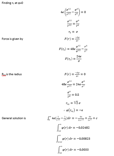
Task 5: Lennard-Jones parameters
r = r*×σ = 1.088 nm
Well depth in LJ potential = -ε = -120×kB J = 1.65677822×10⁻²¹×Na J/mol = 997.735181 J/mol = 0.998 kJ/mol
T = T*×(ε/kB) = 1.5×120 = 180 K
Equilibration
Task 3: Face-centred cubic
Face-centred cubic has 4 lattice points per unit cell. When our box is created it contains 1000 unit cells each with 4 lattice points. Therefore our box contains 4000 lattice points.
NJ: What is the lattice spacing in this case?
NJ: Why can't we use random numbers for the initial positions of the atoms?
Task 4: LAMMPS manual
First line of the command specifies type (1) and mass (1.0) of atom. Second line of the command is used to compute pairwise interactions between atoms, in our case Lennard-Jones potential at a cut-off distance of 3.0 reduced units. Third line of the command specifies pair force field coefficients (1.0 1.0) between all types of atoms (**)
Task 5: Integral type
In our simulation we are going to use Velocity Verlet Algorithm as its the only algorithm that will allow us to compute velocity in the system and therefore calculate kinetic energies.
Task 6: Timestep
We use variable time step line in the command in order to simplify the process of changing the timestep if needed in further simulations. Instead of manually rewriting every command with timesteps, we change one line and code adjusts the rest.
NJ: This section makes sure that you always simulate the same time (nsteps*dt), no matter what timestep is chosen.
Task 7: Energy, Temperature and Pressure
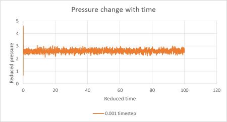
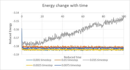
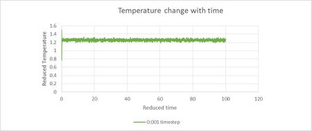
As can be seen from Figures 5-7 and further inspection of data during first 1 reduced unit of time, system does reach equilibrium at around 0.4 reduced time units.
Using Figure 8 we can predict that 0.01 timestep is the highest timestep that will result in successful equilibration of the system and therefore appropriate for our simulation. Higher timestep of 0.015 reduced units is unsuitable due to energy progressively increasing with time. This could be happening due to inaccurate calculations causing system to overshoot at each timestep.
NJ: 0.01 is a bit big. We don't really want the average energy to depend on the choice of timestep - the two smallest timesteps, 0.001 and 0.0025 should give approximately the same results. 0.0025 is then the best choice because we get more time out of the simulation for the same number of steps.
Running simulations under specific conditions
Task 1: Choosing gamma
From rearranging equations 1 and 2 we can obtain that γ2=τ/T
NJ: Show a bit more working.
Task 2: Manual
Argument '100' specifies that values we are calculating will be recorded every 100 timesteps. '1000' argument specifies that average will be taken over 1000 values obtained. And therefore '100000' argument tell the system that 100000 timesteps will be carried out to obtain average value needed.
Task 3: Plotting the equation of State

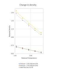
From Figure 6 we can establish that average pressure in our simulation at most accurate timestep of 0.001 is around 2.5 reduced units. Therefore two pressures chosen for density calculations were 2.45 and 2.55 reduced units. Density was measured as 5 different temperatures of 1.6, 1.8, 2.0, 2.2 and 2.4 reduced units at both densities. Resulting Change in Density Graph is presented in Figure 9.
NJ: These error bars seems rather large - are they the Excel default error bars, or the reported errors from the simulation?
Figure 10. shows that the Ideal Gas Equation produces higher density values than our simulation using LJ approximation. Ideal gas equation ignores all intramolecular forces thereby allowing atoms to be packed more closely without any repulsion effect. This results in higher densities than it would in reality. At higher pressures atoms are forced closer to one another and in LJ system atoms will repel and a small change in pressure will not result in a large change in density. Whereas in Ideal Gas approximation atoms are free to arrange as close as possible resulting in an increased discrepancy between LJ and Ideal Gas Law densities at higher pressures.
NJ: What about the trend in the discrepancy with temperature?
Calculating Heat Capacities using statistical physics
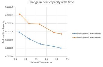
Example input file can be found here File:0.8,2.0.in.
NJ: You shouldn't just join up the points in plots like this - do you think the kink is really part of the trend, or the result of measurement error? You could fit a line or curve instead, if you wanted to.
Presented in Figure 11 is a graph of change in heat capacity over time for our system at 2 different pressures. Trend of the graph is as expected, heat capacity decreases with an increase in temperature. At higher temperatures atoms gain kinetic energy increasing the number of available degrees of freedom allowing a more effective energy transfer through the entity. At higher temperatures higher proportion of particles are in a higher excitation energy state meaning that less energy will be required to excite the whole system. Heat capacity is an extensive property that will be affected by the size of the system. Increase in density results in an increase in a number of particles per unit volume. Larger number of particles require larger energy input in order to be exited and promoted to higher energy levels this therefore results in an increase in heat capacity.
Structural properties and the radial distribution function
Task 1: Lennard-Jones system in three phases
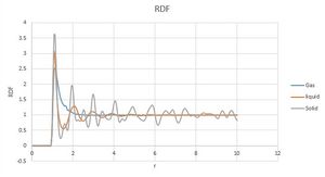
Figure 12 shows Gas, Liquid and Solid radial distribution functions. It is clear from the graph that Gas system has most disorder as only one peak is observed, where most atoms are likely to be found at peak separation r. This is due to random motion of gas molecules. Solid radial distribution on the contrary shows a very high order of a uniform crystal. RD function has multiple peaks throughout the entire range of separation values showing that atoms are in their fixed positions.
NJ: But they oscillate slightly about these positions, that's why the peaks are broad instead of delta functions.
Liquid radial distribution is an intermediate between that of gas and solid. Liquid system is more ordered than gas but less ordered than solid showing that some radial separations are more likely. However unlike in solid system, liquid distribution becomes uniform at higher separation values.
Integrating RDF for all states also confirms that solid system is more ordered than liquid more ordered than gas. Numerical integral of RDF of a solid system is around 4000, liquid 3000 and gas only 200 meaning that all atoms in the solid system are in close proximity to one another, liquid less so and gas atoms are quite far apart from each other. NJ: This isn't about ordering, it just shows that the density is higher in the solid.
Solid system was modelled as a face centred cubic. There are 3 main inner-atom separations in a lattice of such system. Those separations are represented by the first 3 peaks on the RDF graph seen in Figure 12. Shortest separation being 1.125 reduced units representing the distance between face and adjacent corner lattice points. Separation between two adjacent corner lattice points is then 1.605 reduced units. And finally separations between corner lattice point and opposite face centred lattice point is 1.972 reduced units. Therefore lattice spacing is 1.605 reduced units.
NJ: Show these three "neighbours" on a diagram. You can express all three distances in terms of a, the lattice spacing, then use the three distances to get an average estimate for a. Your answer is a little large.

Coordination number of each lattice can be found by estimating area under the RDF curve. This can be done by using graph of integrated RDF of a solid presented small section of which is presented in Figure 13. Peak values labelled on the graphs correspond to the end value of each peak on RDF curve.
Numerical integral of the first peak is 11.83 implying coordination number of 12. This is expected in a face centred cubic as each face lattice point is coordinated to 4 face lattice points above it, around it and below it.
Second peak corresponding to separation between two corner lattice points has numerical integral value of 17.8-11.8 = 6. This corresponds to the predated coordination number of 6, as there are 6 neighbouring corner lattice points.
Third peak representing coordination between the corner and its opposing face lattice points has numerical integral of approximately 42.4-17.8 = 24.6 reduced units. This also agrees with expected coordination number of 24 where each lattice point is coordinated to 3 other lattice points per unit cell. Since each point is in the corner, it will be surrounded by 8 lattice cells and therefore will coordinate with 3*8=24 other lattice points.
Dynamical properties and the diffusion coefficient
Task 1: Mean squared displacement
As expected the MSD of any state system increases with time. It can be seen from Figures 14-16 that vapour systems are much more disordered than liquid and therefore solid systems as previously discussed. Figure 14 shows that MSD of vapour system increases with time and becomes linear at later timesteps. This is because at first atoms start their motion in a straight line translating through space with constant velocity before colliding with one another.
NJ: Excellent. We call this the ballistic regime.
Constant velocty implies that particle displacment is proportional to time and hence MSD is proportional to time squared resulting in parabolic shape of the graph. As soon as first collision occurs atoms gian velocity and randomness in their motion. When all the atoms in the system collided at lease once system starts to follows linear trend in increase of MSD. In solid systems atoms are in fixed positions and are not free to randomly move around, only to vibrate about a fixted position. This first displcement in a vibration is seen as the first spike in the MSD after which molecular vibrations average out and result in almost constant MSD.

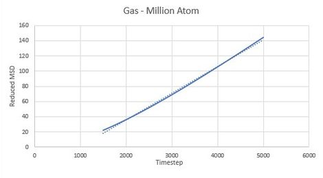

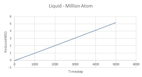
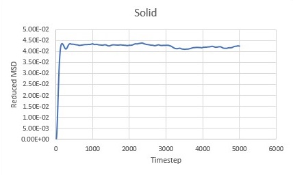

Difussion constns can be calculated by finding the gradient of the linear region of each graph. Results for both Million Atom systems and computed systems can be seen in Table 1.
| Table 1. | Vapour | Liquid | Solid |
|---|---|---|---|
| D | 3.2 | 0.089 | 0.0000083 |
| D for Million Atoms | 3.3 | 0.089 | 0.000025 |
NJ: Do these follow the trend you would expect?
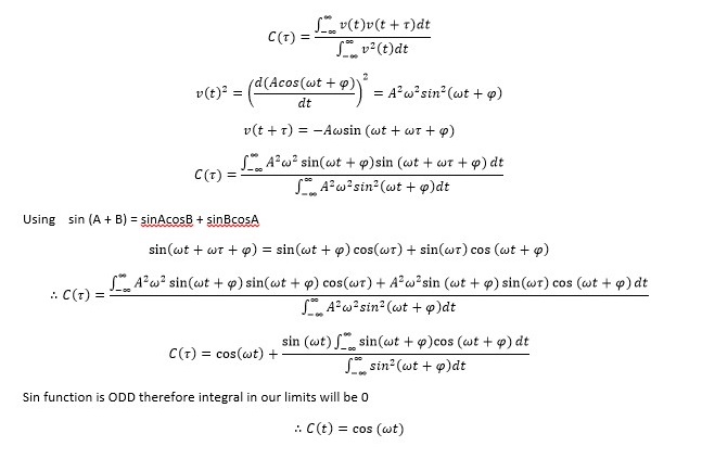
Task 2: Velocity autocorrelation function
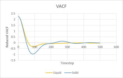
NJ: Where is the harmonic oscillator result? What do the minima represent?
Task 3: Trapesium rule and Difussion coefficient
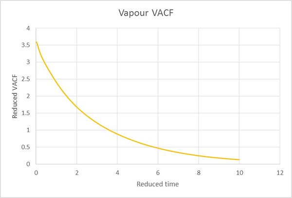
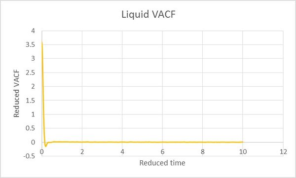
All the D values can be calculated from the numerial intergation of velocity autocorrelation functions. Calculated D values are summarised in Table 2.

| Table 2. | Vapour | Liquid | Solid |
|---|---|---|---|
| D | 2.12 | 0.097 | 0.001332728 |
| D for Million Atoms | 3.27 | 0.09 | 0.00046 |
NJ: How do these compare to your values from the MSD?
