Talk:Mod:DS4113 LIQ

JC: General comments: Make sure that you follow the tasks in the instructions carefully and in order and try to give clear, concise answers. Some tasks were missing or not fully completed.

Chemists often like to think that any property of a system can be calculated using rigid molecules with Monte-Carlo algorithm. For some simulations, however, molecules can no longer be considered rigid in space, and some sort of dynamic evolution with time has to be considered. For such systems, molecular dynamics simulations are a better choice.

JC: There are a large range of situations where molecular dynamics is a much more suitable method than Monte Carlo.

Introduction

Grant and Richards defines molecular dynamics simply as ‘simulation of motions of a system of particles (atoms) with respect to the forces which are present’^[1]. If we consider a system of particles, each at some position, r, and under an influence of some potential field (Lennard-Jones in our case, but there are many others), we can then easily calculate the forces that the particles exert on each other. Using simple Newtonian mechanics, it can be shown that if we know the acting forces and initial velocities/momenta, as well as initial positions, we can calculate a dynamic evolution of the given system with time:

If we compare this result to the Taylor series for discplacement:

We can mention, that our solution only contains the first 3 terms, but not the rest. Generally, our solution is correct for infinitesimally small time-steps, but as the time-step gets bigger, this introduces some level of errors.^[1]

Also, we assume that during the whole duration the step, the acceleration is constant, which, once again, introduces some errors. This error can be reduced either by using smaller time-steps, or, for example, using a so-called Leapfrog Verlet method^[1]

The Leapfrom Werlet method calculates the avegare acceleration between t –dT and t+dT :

As $a = F / m$ , we can substitute back into the first equation to get:

In this equation, we don’t use both velocity and acceleration at the same time, which minimizes the errors.^[1]

Since we are calculating the properties on limited scales, it is advised to use periodic boundary condition to ensure the potential is approximately constant throughout our chosen simulation box.

Generally, the dynamic simulations are conducted under certain temperature. If we want to translate this requirement into our calculations, we must first model the system, minimize its energy, and then heat up the system the the required temperature. The temperature of the system is calculated using the equipartiton theorem:

As at the start of the simulation, we have no information about the initial velocities. The algorithm distributes them randomly using the Bolzman distribution. The system will go through a few steps before reaching the desired temperature. It is also important to state that even when the system this temperature, the temperature will still fluctuate.

Practical example

As mentionad in the introduction, the dynamic simulations often introduce some level of errors. To examine this further, a simple simulation of a classical harmonic oscillator had been set up. The results of applying the Verlet algoritm were compared to a classical solution. Results can be seen in Fig. 1.

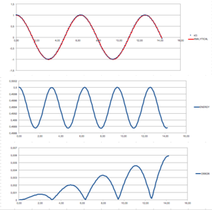
At first, the position using a classical equation was calculated : $X = A c o s (ω t + ϕ)$ . This was then compared to the position obtained using the Verlet algorithm by calculating absolute the value of the difference between the two results. We can see that the behaviour of our ‘error function’ is somewhat periodic, the reasons for this behaviour shall be discussed later on. The time at which the maxima occurs was then plotted with respect to the ‘order’ of the maxima (starting from 0), to get following linear equation: $T I M E = 3.04 * O R D E R + 1.94$ When, however, compared to how the energy (of the Verlet solution) depends on time, we can see that this position of the maxima in the error function correspond the the minima of the energy function. This results from the fact that the classical solution states that the energy of our system should remain constant (0.5 units), but in the Verlet solution, the energy slightly oscillates (maxima at minimum velocities, minima at maximum velocities). From this observation, we could, strictly mathematically, determine expected the position of the error maxima as the positions of the maximum velocitities. Using classical mechanic, this gives:

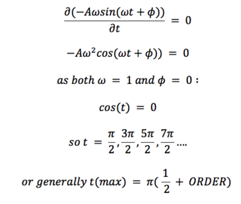
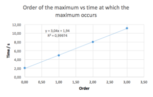
We can see that this result is different from our solution using the Verlet algorithm. This is mainly due to the 0^th order being at a slightly shifted position. If we do not include the 0^th order maximum, and plot the order vs time, we can obtain a great linear fit (R2 = 1) with the equation resembling the theoretically-obtained one much closely. Needless to say, fitting a function into only three points is not a good practice. Here, it was only used to prove that the behaviour of the error function could perhaps be explained theoretically, and to get a meaningful results, an examination of the behaviour of the maxima at higher orders would be needed.

The actual values of the error maxima vs the order of the maxima were also plotted. Linear function $V A L U E = 0, 0013 * O R D E R + 0, 0007$ was then fitted (R2 = 0.99991). This again resembles a function of a form $Y = C O N S T * (1 / 2 + O R D E R)$ . This is interesting because we can clearly see that the error gets larger with each oscillation, and could be perhaps due to the fact that the behaviour of our system is dependent on its state in the past, and as each step carries a certain error to itself, it is reasonable that this error is going to be higher each cycle we perform. It is therefore appropriate to monitor the energies and positions when modelling a physical system numerically to ensure the system does not 'misbehave' in any way.

The Lennard-Jones Potential

As mentioned in the introduction, to calculate the force that influeces each atom, Lennard-Jones potential was used.

For a single interaction, potential is of a following form:

The potential tends to 0 as r increases to infinity.

JC: Where does the potential cross zero? - This is r0. What is the force at r0?

The minimum of this potential can be found by differentiation:

JC: Correct

And finally, the well depth of the LJ potential is:

JC: The well depth should be -epsilon, not -2*epsilon, (1/4 - 1/2 = -1/4).

As it would be computationally very demanding to calculate the interaction energy for each and every atom, we can approximate that after certain length, the potential becomes essentially zero, and so we can neglect interactions with particles outside the sphere of a given radius. This radius should be smaller that half of the length of our box to make sure we do not calculate any interaction twice (this results from periodic boundary conditions). For practical example, the integrals under the LJ curves were calculated from infinity to $3 σ$ , $2.5 σ$ and $2.0 σ$ . The values (in reduced units) obtained were $- 3.3 * 1 0^{- 3}$ , $- 8.2 * 1 0^{- 3}$ and $- 0.025$ . We can see that all the values are very small, but if possible using larger cut-off distance should give more accurate results as the introduced error is smaller.

JC: Integrals are correct.

Reduced units

It is often the case that computational chemists use so-called reduced units. This means that the quantities used for the simulations are divided by convenient scaling factors to obtain more manageable numbers, typically in order of units, tens,.. To recognise we use reduced units, their symbols are usually denoted by star. For example:

$E^{*} = E / ϵ$

For argon, $σ = 0.34 n m$ and $ϵ / k_{B} = 120 K$ , the cut-off (in reduced units) is 3.2 and the temperature (in reduced units) is 1.5, then the cut-off is S.I. units is 3.2*0.34 nm = 1.088 nm and the temperature of the system in S.I. units is 1.5*120 = 180 K. We can also calculate the L-J potential well depth as $- 2 ϵ = - 2 ϵ / k_{B} * k_{B} = - 240 k_{B}$

JC: Cut off and temperature are correct. The well depth is epsilon, you need to convert this into kJ/mol.

Periodic boundary conditions

As mentioned above, for often we use so-called periodic boundary conditions. This is due to the fact that simulating systems at macroscopic levels would be absurdly computationally demanding. For example, 1 mL of water at room temperature contains approximately $3 * 1 0^{22}$ molecules! Trying to calculate all the interactions, even with relatively shor cut-off distances would be impossible. It is often the case that we can simulate the behaviour using tens of thousands molecule (which corresponds to approximately $3 * 1 0^{- 19} m L$ !!) and get data that perfectly fits experimental data acquired at macroscopic amounts of material. This is done by constructing a cell which is in contact with the exact replicas of the initial cell. This ensures that the species at the border of the cell experience the same potential as these in the very centre of the cell. To ensure the number of particles stays constant, whenever a particles leaves a cell, another particles enters the cell through the opposite face of the cell. For example, if we have a particle at [0.5, 0.5, 0.5] in a cubic cell (a = 1.0), and this particles moves by (0.7, 0.6, 0.2), which results in the particle leaving the cell (new position is [1.2, 1.1, 0.7]), another particle enters the cell and ends up at [0.2, 1.1, 0.7].

JC: Periodic boundary conditions are used to remove the interfaces around a simulation box and allow simulations to probe bulk properties without being dominated by interfacial effects. The particle should end up at (0.2, 0.1, 0.7), it exits both the x and y edges of the box and returns through the opposite faces.

Time-step

When conducting a calculation, it is importnant to decide what time-step to use. Generally, larger steps allows the system to equilibriate quicker (less steps needed), but, as discussed above, introduces some errors, which can even become significant (at large enough time-steps). Using smaller time-steps results in both more accurate and more precise results, but the system takes longer to equilibrate. It is also more time-demanding to run the simulation for longer times, as the number of steps needed to calculate is larger. It is therefore important to find a balance between these two extremes.

To back up these conclusions, a sc system of density 0.8 was set up. A sc lattice of density 0.8 has lattice spacing of 1.07722 as

$ρ = m / V$ , where m = 1 as the mass of the particles is 1 and there is 1 particle per cell in sc

$V = 1 / ρ$

We know that $V = (s p a c i n g)^{3}$ so $(s p a c i n g) = V^{1 / 3}$ ,

And finally

$a = (1 / ρ)^{1 / 3} = 1.07722$

If we, for example, were dealing with a fcc lattice with density of 1.2, there are 4 particles per unit cell, so

$a = (4 / 1.2)^{1} / 3 = 1.494$

10 lattice cells were then created in each direction, resulting 1000 cells so the system contains 1000 particles. If the system was, for example, created using fcc cells, it would contain 4000 particles instead as there is 1000 cells, each containing 4 particles.

JC: Correct.

It is important to start with ordered particles (in our case each particle occupies one site in the sc lattice), rather than to give the particles a random starting coordinates to assure that no particles are places too close together, which could result in anomalous behaviour of the system.

JC: What sort of anomalous behaviour?

Velocities were then randomly distributed using the Bolzmann distribution, and number of simulation were run using the velocity (Leapfrom) Verlet algorithm, each with a different time-step.

The command:

### SPECIFY TIMESTEP ###

variable timestep equal 0.001

variable n_steps equal floor(100/${timestep})

variable n_steps equal floor(100/0.001)

timestep ${timestep}

timestep 0.001

### RUN SIMULATION ###

run ${n_steps}

run 100000

was used, rather than a simpler

timestep 0.001

run 100000

to ensure the simulation initially runs for the same time, independent on value of the time-step.

In figure 3, the energy of our system system is plotted as a function of number of steps. We can see that for 0.1 ps time-step, the system equilibrates relatively easily, but then fluctuates around its average values quite widely. It can also be seen that the average value of energy is somewhat higher then for the other cases.

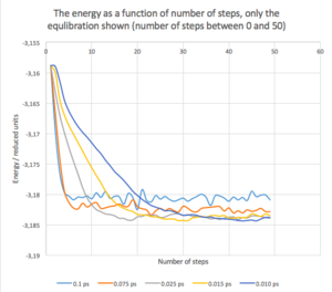
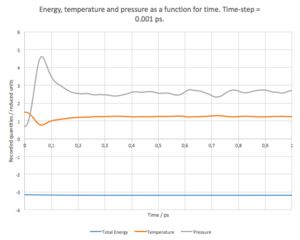
On the other hand, for the 0.01ps time-step, the system has to undergo more steps to reach the equilibrium, but once the equilibrium is reached, the system does not vary to much with respect to the average value. We can also expect that the value of the system’s energy is more accurate. As expected, the time-steps between these two extreme cases shows a mixed behaviour between the two, gradually changing from one to the other, as the time-step is increases/decreases. Temperatures and pressures for each system were recorded as well. The dependence of energy, temperature and pressure as a function of time (time-step = 0.001 ps) can be seen in Fig. 4. It can be seen that the energy equilibrates quite fast, but it takes about 0.2 - 0.3 ps for both the pressure and the temperature to equilibrate as well.

JC: What timestep did you choose and why? Extending the range of the x axis in the time vs total energy plot may also help you to choose.

The calculations also returned trajectory files that were animated using VMD. The periodic boundary conditions could be clearly observed when two particles were enlarged to focus on their paths.

The NpT ensamble

The simulations above were done holding N, V, and E constant. However, sometimes we need to keep other quantities constant. In this part of the computational exercise, the number of particles, the pressure and the temperature were held constant, allowing V to freely equilibrate.

The simulations were run 10 times, each time at different conditions (two different pressures (2.5 and 3.0) each at 5 different temperatures (1.6, 1.7, 2.0, 2.3 and 2.5). The system was allowed to equilibrate and then its pressure, temperature and density were recorded by a following command:

### MEASURE SYSTEM STATE ###
thermo_style custom step etotal temp press density
variable dens equal density
variable dens2 equal density*density
variable temp equal temp
variable temp2 equal temp*temp
variable press equal press
variable press2 equal press*press
fix aves all ave/time 100 1000 100000 v_dens v_temp v_press v_dens2 v_temp2 v_press2
run 100000

The three numbers, 100 1000 100000 tell the program how to collect the data; 100 1000 100000 tells the program to calculate the average every 100000 steps using 1000 values with 100 steps in-between each value. This effectively means that the average was calculated every 100000 steps using the values at the 100th, 200th, 300, 400th, ....., 100000th step.

The results (with error bars) can be seen bellow.

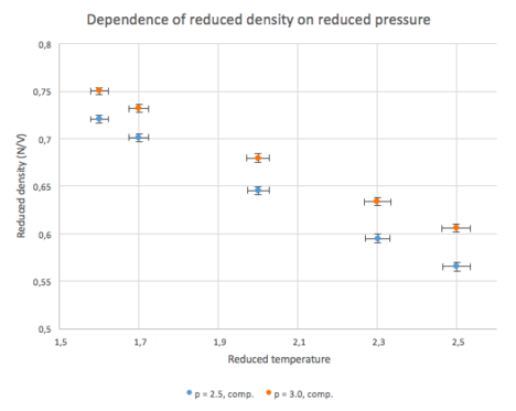
We can see that the behaviour of the system is as expected; at higher pressure, the systems exhibits higher densities, also the reduces density is approximately reversely proportional to the reduced temperature.

As the pressures were high, significant deviations from the Ideal gas law can be expected. For comparison, bellow is the same graph, this time with the reduced densities calculated using the Ideal-gas equation.

Not surprisingly, the deviation from the ideal gas behaviour is larger from the system with higher pressure.

The density is much smaller than expected using the simple ideal gas law, possibly because at the high pressures under investigation, the repulsive term in the L-J potential becomes more dominant and thus the volume of the system is higher compared to the result obtained simply by taking pV = nRT.

JC: Good comparison with ideal gas.

The heat capacity

The heat capacity of our system at a particular temperature can be calculated using statistical mechanics as

$C = \frac{\partial ⟨ E ⟩}{\partial T} = - \frac{β}{T} \frac{\partial ⟨ E ⟩}{\partial β} = \frac{β}{T} \frac{\partial^{2} \ln Z}{\partial β^{2}} = \frac{β}{T} \frac{\partial (\frac{\partial Z}{Z \partial β})}{\partial β} = \frac{β}{T} (\frac{\partial^{2} Z}{Z \partial β^{2}} - (\frac{\partial Z}{Z \partial β})^{2}) = \frac{β}{T} (⟨ E^{2} ⟩ - {⟨ E ⟩}^{2})$

As the program collects the energies per particle, this has to be further multiplied by N*N (N is the number of particles) to obtain the absolute value for our system.

The data needed were collected using following script:

### DEFINE SIMULATION BOX GEOMETRY ###

variable D equal 0.2

lattice sc ${D}

region box block 0 15 0 15 0 15

create_box 1 box

create_atoms 1 box

### DEFINE PHYSICAL PROPERTIES OF ATOMS ###

mass 1 1.0

pair_style lj/cut/opt 3.0

pair_coeff 1 1 1.0 1.0

neighbor 2.0 bin

### SPECIFY THE REQUIRED THERMODYNAMIC STATE ###

variable T equal 2.2

variable V equal 1/${D}

### As VOLUME = MASS over DENSITY, and in our case MASS = 1 ###

variable timestep equal 0.0005

### ASSIGN ATOMIC VELOCITIES ###

velocity all create ${T} 12345 dist gaussian rot yes mom yes

### SPECIFY ENSEMBLE ###

timestep ${timestep}

fix nve all nve

### THERMODYNAMIC OUTPUT CONTROL ###

thermo_style custom time etotal temp press

thermo 10

### RECORD TRAJECTORY ###

dump traj all custom 1000 output-1 id x y z

### SPECIFY TIMESTEP ###

### RUN SIMULATION TO MELT CRYSTAL ###

run 10000

unfix nve

reset_timestep 0

### BRING SYSTEM TO REQUIRED STATE ###

variable tdamp equal ${timestep}*100

variable Vdamp equal ${timestep}*1000

fix nvt all nvt temp ${T} ${T} ${tdamp}

unfix nvt

fix nve all nve

run 100000

reset_timestep 0

### MEASURE SYSTEM STATE ###

thermo_style custom step etotal temp press density

variable temp equal temp

variable temp2 equal temp*temp

variable en equal etotal

variable en2 equal etotal*etotal

fix aves all ave/time 100 1000 100000 v_temp v_temp2 v_en v_en2

run 100000

variable avetemp equal f_aves[1]

variable errtemp equal sqrt(f_aves[2]-f_aves[1]*f_aves[1])

variable heatcap equal ((f_aves[4]-f_aves[3]*f_aves[3])/f_aves[1]*f_aves[1])

print "Averages"

print "--------"

print "Temperature: ${avetemp}"

print "Stderr: ${errtemp}"

print "Heat_cap: ${heatcap}"

At first, a system containing 15*15*15 sc cells was created. It was then allowed to equilibrate under the prescribed conditions and then the state of the system was recorded and E, E2, T and T2 were extracted. The heat capacity was defined without the N*N term, so the obtained values then had to multiplied by 15^6.

The heat capacities were then measured tor 10 different systems, and the results can be seen bellow.

	T(init) = 2.0	T(init) = 2.2	T(init) = 2.4	T(init) = 2.6	T(init) = 2.8
density = 0.2	0.6767	0.84458	0.4565	0.59675	0.5385
density = 0.8	0.4033	0.4423	0.3899	0.3794	0.3616

After examining the output files, it was mentioned that is the temperature of the system was free to change, the values of T were different from the ones used to set the experiment up. After taking this into consideration, and dividing the absolute values of the heat capacity by the volume of the system, a following graph was produced (density = 0.2 in blue, density = 0.8 in orange):

JC: Temperature will fluctuate, but should fluctuate around a constant value. Is this plotted for the temperature of the final step of the simulation?

We can clearly the a peak in Cv/V for both systems, this could indicate a phase transition, but the system would have to be sampled better (more samples around the critical values) to fully conclude that. What even more interesting is that the peak occurs at the same initial temperature for both systems:

JC: Joining up the data points in the graph with a smooth line is misleading as there is no reason why the heat capacity curve should follow this line between the data points.

This could indicate that the initial states of the system, before the data for calculating Cv were collected, could undergo the mentioned phase transition.

The value of Cv/V is generally higher for the 0.8 system, which is physically reasonable, as there are more atoms per unit volume, requiring more energy to change the temperature of the sample.

The radial distribution function

Radial distribution function, g( r), is a function that shows the variation of density in the system with distance from a particular point in the system. Mathematically it is defined as follows:

Where N( r) is the mean number of atoms in a shell of thickness delta r at distance r, and rho is the atom density.

The significance of the function results from the fact that it can link macroscopic and microscopic properties using the Kirkwood-Buff solution^[2]. Solid (reduced density = 1.4, reduced T = 1.2), liquid-like (reduced density = 0.7, reduced T = 0.3), gas-like (reduced density = 0.1, reduced T = 0.8) and fluid (reduced density = 0.4, reduced T = 2.0) systems were modelled (time-step = 0.0002 ps) and allowed to equilibrate, after which their radial distribution functions, as well as the integrals of the RDFs, were calculated using VMD. The RDFs for all systems can be seen in Fig. 5.

JC: You should have chosen densities and temperatures to simulate a pure solid, liquid and gas.

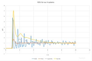
As a general trend, g(r) is zero when r < 1, after that it rises rapidly.^[2] This can be explained by the facts that we simulate the particles as hard spheres, so there can be no particles in the region smaller then the radius of the species with respect to which the g(r) is measured. The first peak is generally the global maximum because the $4 π r^{2}$ term is much smaller compared to higher order peaks.

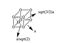
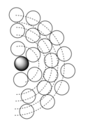
Let’s look at the solid phase first. We can see many peaks, seemingly randomly distributed. The fact that g(r) does not approach 1 fast, as in the other examples, indicates long-range order. ^[3]Each peak can be correlated to particular neighbours of any given point in the lattice. For example, the first peak (with highest g(r)) can be correlated to the closest neighbours in the fcc structure, two second to the second closest, etc.. This can be seen in Fig. 6. There is 12 pairs of species at the closest distance, 6 at the second closest and 24 at the third closest.

JC: Good idea to include a diagram of the fcc structure. Did you plot the integral of the RDF? This can be used to confirm the number of atoms responsible for each peak in the RDF.

As shown in Figure 6., the second peak corresponds to the lattice spacing, a. From g(r), the lattice spacing should correspond to the second peak, and thus should be 1.425. Since the density of our system is kept close to 1.4, the spacing can also be calculated:

$D e n s i t y = (4 / 1.4)^{1 / 3} = 1.419$

We can see that the values are in reasonable agreement, the small difference stems from the fact that the calculation of g(r) had been done with 0.05 increments in r, and should the increments be smaller, more accurate value would be obtained.

The g(r) for the fluid, one-phase region shows one peak, a small minimum and then rapidly approaches 1. This is something to be expected from a gas-like phase. The first, and only, peak corresponds to species close to the particle in question, they form a sphere around the particle. This does not necessarily indicates any pronounced interactions between the particles, but could stem from purely geometrical considerations, as that small distances, even in disordered systems, there will always be some close neighbours to each species. After that, the structure becomes disordered and the function approaches 1 rapidly. ^[2]

The third and fourth system configuration were chosen to be in the G+L region. The third one is in region that should exhibit more liquid-like behaviour, the fourth should shoul more gas-like behaviour.

JC: You should have simulated a pure gas and pure liquid, not configurations in the coexistence region.

It can be seen that in the third example, g(r) somewhat oscilates around g(r) = 1, and eventually approaches g(r) = 1 at high enough r. This is typical for liquids. In simple terms, if we stack hard spheres, there is always going to be radii with higher densities and ones with lower densities. Fig. 7. Could perhaps make this point a bit clearer.

Finally, for the fourth case, it can be mentioned that is shows a mixed behaviour between gas and liquid. g(r) decreases rapidly towards 1, showing no medium- or long- range order, but shows 2 peaks corresponding to some level of short-range order, perhaps even a hydration-like spheres.

The integrated forms of g( r ) grew as expected, showing a few peaks for smaller r and then grew linearly with r at larger value of r.

The diffusion coefficient

MSD

To quantitatively study how molecules in our sample move, we can use some properties of that system, like for example mean square displacement, to calculate the diffusion coefficient.

In his studies of Brownian motion, Albert Einstein found that the mean squared distance each particle travelled is linearly proportional to the time period in which the motion occurred. Mathematically

$< r^{2} > = 6 D t + C$

Where D is the diffusion coefficient and C is a constant we are not interest in, because if we differentiate this equation with respect to time, we obtain

$D = (1 / 6) d (< r^{2} >) / d t$

which allows us to directly calculate the diffusion coefficient from our calculations.

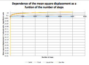
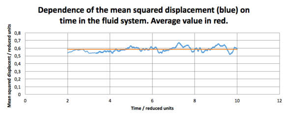
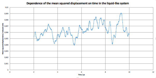
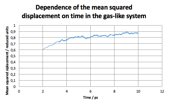
Calculations were set up for each of the 4 system discussed above to obtain the mean squared displacement of each system. In Fig 8, the relationship between the number of steps and $< r^{2} >$ is shown. We can mentioned that initially the system starts with very small $< r^{2} >$ and it takes about 2000 steps for the system to equilibrate, thus for further calculation, only steps higher than 2000 were taken into account.

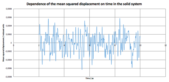
Below, D as a function of time for each of our system can be seen.

JC: You should also include the linear fits to the MSDs that you used to calculate the diffusion coefficients on your graphs.

JC: The liquid-like system looks more like a solid based on both the MSD and RDF.

Looking at each system separately, it can be seen that the value of D for the solid system fluctuates around its average value $- 4.36 * 1 0^{-} 7 (\pm 0.00021) σ^{2} / p s$ . This is due to the periodic vibrational motion of the particles in the lattice. As expected, however, the averaged value of D is close to 0 as we do not expect any significant motion of the particles in the lattice.

For the second system, the in the fluid state (resembling the gas phase, as found above), D was found to be $0.5833 (\pm 0.0319) σ^{2} / p s$ .

The diffusion coefficient for the third system, resembling the liquid state, was found to be $0.00627 (\pm 0.00107) σ^{2} / p s$ . This again support the assumption made before that the system can be considered liquid, as the diffusion coefficient is almost 100-fold smaller!

Interestingly, in the fourth case, the system had not reached the equilibrium even after 5000 steps, so the value of the diffusion coefficient for this system was not calculated. It can be seen, however, that the value approaches approx. 1, which is something to be expected from a gas. The value is greater that of the second system due to system 4 having lower density, thus allowing for higher mean free path.

The diffusion coefficients were also extracted from data provided for simulations with million particles. The data, however, did not include any information about the time-step, so the diffusion coefficients presented in this section are taken with respect to the number of steps , rather than time. To get the actual value of the coefficients, they need to be devided by the value of the time-step used.

Similar behaviour to our simulation can be mentioned. For the solid phase, D(wrt steps) = $- 9.228 * 1 0^{- 9} (\pm 1.050 * 1 0^{- 7}) σ^{2}$ , again close to zero. The coefficient w.r.t. steps for liquid phase was calculated to be $0.000177 (\pm 2.059 * 1 0^{- 6}) σ^{2}$ , and the one for the vapour phase is reaching values of approximately 0.006-0.007. As the system, again, did not equilibrate within the number of steps performed, only an approximate value is presented. Nevertheless, it can be again mentioned that the value is larger that that for liquid.

To compare results, the value of the time-step for the given results would be needed. Even though, we can still see that the general trend D(solid) < D(liquid) < D(gas), and for both sets of data D(gas)/D(liquid) is of order of $1 0^{2}$ and D(liquid)/D(solid) in order of $1 0^{4} - 1 0^{5}$ .

It can be seen that although the diffusion coefficients are somewhat different, at least their relative magnitudes are the same.

VACF

The diffusion coefficient can also be calculated using the velocity autocorrection function:

$C (τ) = ⟨ v (t) \cdot v (t + τ) ⟩$

D can then be calculated as

$D = \frac{1}{3} \int_{0}^{\infty} d τ ⟨ v (0) \cdot v (τ) ⟩$ The VACF tells us how much the velocity change with respect to the initial velocity after some time-step.

For the reasons mentioned above, we can expect the VACF of a simple harmonic oscillator to strongly correlate with its acceleration.^[4]

The VACFs were extracted from our simulations of liquid and solid, and additional VACF for a harmonic oscillator (omega = approximately 0.1) is included as well. We can mention that for solid, the VACF oscillated widely, while exponentially decaying, behaving practically like a damped oscillator. This is because the of the vibrational motion of atoms in the lattice. The decay is caused by the fact that this vibration is not perfectly harmonic, but there are some pertubative forces that disrupts the 'perfection' of the motion. For liquid, we can see one minimum, after which the function decays to 0. We expect the diffusion to destroy any signs of vibrational motion, this results in the function being close to zero. The minimum in the function can be considered as a collision between two particles (so there is some correlation between their velocities), after which they rebound and by the diffusive forces, the VACF becomes 0 again. This behaviour is similar to a strongly damped oscillator.

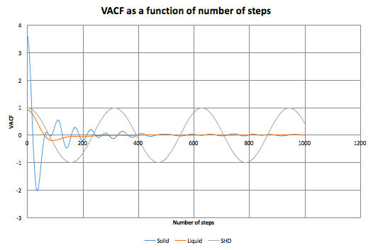
For the solid and liquid systems, the integrals were evaluated numerically (in the region 0-500 time-steps, as the contribution at higher time-steps should become negligible), and using these values, their diffusion coefficients were calculated. For solid,

D = 0.000103 σ^{2} / p s

, and for liquid

D = 0.007374 σ^{2} / p s

. Again, D(liquid) is higher than D(solid). However the ratio between them is much smaller the the one obtained using the MDS method. The difference stems from the fact that, using MDS, D was calculated in the region after equilibration, but using VACF, D was calculated over the whole region. If D was calculated again in the region between 2000-5000 steps, it would result in D much closer to 0. The two results for the liquid systems compare very well.

JC: What about the vapour phase? You should include plots of the running integrals of the VACFs that you used to calculate the diffusion coefficients.

Conclusions

In this exercise, The effect of different time steps on the results of the calculations was examined. It was found that smaller time-steps result in higher accuracy, but it takes more steps for the system to equilibrate. In the next part, a simple gaseous system was modelled and the dependence of its density on its pressure was examined. The results were then compared to results given by the ideal gas equation. It was found that the densities (for the same pressures) were lower than expected for the IGL. This was attributed to the existence of the repulsive forces at high enough pressures, which is something IGL does not account for.

In the next part, heat capacities as functions of temperature were calculated. The capacities showed a peak, possibly because the system was undergoing a phase transition.

In the next part, the RDF for 4 different systems was calculated. For the solid system, the RDF showed a number of peaks, corresponding to a highly ordered structure. The first 3 peaks were correlated to the actual distances in the fcc structure. The RDF for a liquid showed fewer peaks with approximately the same specing, suggesting an existence of many hydration shells. The RDF for the gaseous system showed only one peak - the closest neighbours - after which there was no order in the system, thus g( r) averaged to 1.

In the last part of the exercise, the diffusion coefficient for each system was calculated using 2 methods - MSD and VACF. Both methods yielded approximately the same results.

Should I repeat the experiment again, I would examine the behaviour of the NPT system at lower pressures to see whether the calculated density would be higher then expected (due to attractive forces this time). I would also run more configurations in the Heat capacity part of this experiment to perhaps find the coexistence curve.

Literature sources

↑ ^1.0 ^1.1 ^1.2 ^1.3 Grant, Guy H, and W. G Richards. Computational Chemistry. Oxford [England]: Oxford University Press, 1995. Print.
↑ ^2.0 ^2.1 ^2.2 Nijboer, B. R. A., and L. Van Hove. "Radial Distribution Function Of A Gas Of Hard Spheres And The Superposition Approximation". Phys. Rev. 85.5 (1952): 777-783. Web.
↑ Yoon, B. J., M. S. Jhon, and H. Eyring. "Radial Distribution Function Of Liquid Argon According To Significant Structure Theory". Proceedings of the National Academy of Sciences 78.11 (1981): 6588-6591. Web.
↑ Tuckerman, Mark E. Statistical Mechanics. Oxford: Oxford University Press, 2010. Print.

[:0-1] 1.0 ^1.1 ^1.2 ^1.3 Grant, Guy H, and W. G Richards. Computational Chemistry. Oxford [England]: Oxford University Press, 1995. Print.

[:1-2] 2.0 ^2.1 ^2.2 Nijboer, B. R. A., and L. Van Hove. "Radial Distribution Function Of A Gas Of Hard Spheres And The Superposition Approximation". Phys. Rev. 85.5 (1952): 777-783. Web.

[3] Yoon, B. J., M. S. Jhon, and H. Eyring. "Radial Distribution Function Of Liquid Argon According To Significant Structure Theory". Proceedings of the National Academy of Sciences 78.11 (1981): 6588-6591. Web.

[4] Tuckerman, Mark E. Statistical Mechanics. Oxford: Oxford University Press, 2010. Print.

[1]

[2]

[3]

[4]