Talk:Mod:DMS3053

CMP Programming Experiment - Daniel Spencer, 00736964

Introduction to the Ising Model

Minimum energy of the Ising Model

Using the equation

E = - \frac{1}{2} J \sum_{i}^{N} \sum_{j \in n e i g h b o u r s (i)} s_{i} s_{j}

(eq. 1)

the minimum energy of an Ising lattice of $D$ dimensions, with $N$ spins (where each spin had a value of +1 or -1) and an interaction strength of $J$ was considered. This was achieved first through a consideration of a one-dimensional system with five parallel spins (where the spins are parallel as this corresponds to the minimum energy arrangement of the system). Hence, the energy of this linear system was found to be

E_{min,1D} = - 5 J

.

For a linear, one-dimensional system, the number of neigbouring spins is two. The number of neighbours can be determined for two- and three- dimensional systems through a geometric consideration of their structure - the values are presented in Table 1.

*Table 1: Dimension numbers and number of neighbours*
Number of Dimensions, D	Number of Neighbours
1	2
2	4
3	6
D	2D

These data indicate that the number of neighbours is twice the number of dimensions, for the dimensions considered here. This can be extrapolated to give the general number of neighbours as $2 D$ .

For the minimum energy of the system, where all spins are parallel, every combination $s_{i} s_{j}$ has a value of 1. Notably, for each value of $i$ , there will be $2 D$ neighbour interactions. Ergo, using eq. 1, the general minimum energy can be found to be

E_{min,D} = - D N J

(eq. 2).

To check this equation, it can be applied to the two-dimensional Ising lattice with 25 spins - this gives a value of

E_{min,2D} = - 50 J

,

which matches with the value predicted from first-principles.

For this D-dimensional system, the multiplicity (i.e. the number of ways of achieving the specified configuration of spins) must be equal to two, as either all of the spins could be aligned 'up' (+1) or 'down' (-1). Using this multiplicity, the entropy of the system can be calculated using the equation

S = k_{B} \ln Ω

, (eq. 3)

where Ω is the number of microstates (equal to the multiplicity in this case), which gives a value of $k_{B} \ln 2$ , or 9.57 x 10^-24 J K^-1.

NJ: good.

Spin 'flipping'

**Figure 1**: Representation of Ising lattices in one (N=5), two (N=25), and three (N=125) dimensions. +1 and -1 spins are denoted by the red and blue cells respectively. Diagram taken from the lab script.

Using the Ising model, it is also possible to consider a change in state, reflected by a 'flipping' of the direction of one of the lattice spins. For this case, the energy (using eq. 1) can be determined to be

E^{'} = - \frac{1}{2} J (2 D N - 4 D - 4 D) = 4 D J - D N J

, (eq. 4)

where the additional $4 D$ terms arise from the loss of 4D stabilising spin-aligned interactions and the gain of 4D destabilising spins anti-aligned interactions following spin 'flipping'. Using eq. 2 and eq. 4, the change in energy derived from this spin 'flip' can be calculated to be

Δ E = 4 D J - D N J + D N J = 4 D J

. (eq. 5)

For a system with three dimensions (D = 3) and 1000 spins (N = 1000), the system, using eq. 5, was determined to increase in energy by $12 J$ . Notably, this change in energy is independent of the number of spins in the system - it depends only on the number of dimensions and J.

A significant consideration with regards to the spin 'flipping' described here is the accompanying increase in entropy - the driving force for this process. For the scenario describing the change in direction of a single spin, the multiplicity of the system will be $2 N$ - this is a consequence of the system prior to 'flipping' having a multiplicity of two (all spins aligned 'up' or 'down'), where now, any one of the spins could flip, adding the factor of N to the multiplicity. Hence, the new entropy can be defined to be

S^{'} = k_{B} \ln 2 N

, (eq. 6)

which allows the change in entropy to be calculated according to eq. 7.

Δ S = k_{B} \ln 2 N - k_{B} \ln 2 = k_{B} \ln N

(eq. 7)

For the system described above (D = 3, N = 1000), the change in entropy associated with the spin 'flip' process is therefore $k_{B} l n 1000$ , which is equal to 9.53 x 10^-23 J K^-1.

NJ: nicely explained.

Magnetisation

*Table 2: Ising lattices and magnetisations*
Ising Lattice	Magnetisation
1D - spins as in Figure 1	1
2D - spins as in Figure 1	1
3D at 0 K	1000 or -1000

Figure 1 shows three examples of Ising lattices, with one, two and three dimensions respectively. Using the equation for magnetisation (eq. 8), the magnetisations of these systems can be calculated to be those presented in Table 2.

M = \sum_{i} s_{i}

(eq. 8)

For the three-dimensional system with 1000 spins at a temperature of 0 K, all of the spins must be aligned either 'up' or 'down', as the entropic increase associated with 'flipped' spins does not provide a driving force at absolute zero - the only factor to consider is that of the energy, which is a minimum when all of the spins are aligned. For this case, the magnetisation could be either 1000 or -1000, depending upon the direction of the spin alignment. From a consideration of the magnetisation values calculated here, it is evident that with all of the spins aligned, the (magnitude of the) magnetisation of the system is at a maximum.

Calculating the energy and magnetisation

Modifying the files

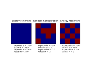
In order to use Python to compute the energy and magnetisation for a given two-dimensional Ising lattice, the class IsingLattice was used, where energy() and magnetisation() functions were written to calculate their corresponding properties for a random numpy array of spins (generated using np.random.choice). For this aspect of the experiment, the value of J was assumed to be 1.0, working in reduced units. The Python script developed can be viewed here, including annotations.

NJ: could be a little simpler (do you need to check every edge case? Good otherwise. Try to make your comments less a description of the Python code, and more a description of the algorithm.

Testing the files

In order to test the script prepared thus far, the Ilcheck.py script was run, generating the image presented in Figure 2. An examination of this output clearly indicates that the script provides accurate energies and magnetisations for the minimum and maximum energy configurations, along with for an intermediate, random arrangement. Hence, it can be concluded that at the current level, the Python script is functioning as required.

Introduction to the Monte Carlo simulation

Average Energy and Magnetisation

**Figure 3**: Animation result from ILanim.py, showing the resting of the system in the minimum energy state

In order to consider the generalisability of the prepared script, it is important to analyse how the script will function for large systems, such as those with 100 spins in the spin array. As each of these spins can be either 'up' or 'down', each spin has two choices. Hence, the number of possible configurations for the system can be written as $2^{100}$ , which has a value of 1.2677 x 10³⁰.

If one considers the sampling of a single configuration to take 1 x 10^-9 s, then it is clear that sampling all of these configurations would take a total of 1.2677 x 10²¹ s (also expressed as 4.017 x 10¹³ years). From this analysis, it is evident that the sampling of configurations was a significant consideration in the writing of a python script for this task.

In order to account for this, the technique of importance sampling was implemented, using the statistical Boltzmann distribution, $\exp (- Δ E / k_{B} T)$ . Note that as the energy computed using the energy() function is in units of k_B, this factor is not included in the script.

Modifying IsingLattice.py to Implement a Monte Carlo Cycle

The python script developed at this stage is presented here, accompanied by annotations to explain how the script functions.

Simulating the Monte Carlo Cycles

*Table 3: statistics() output for animated system at global minimum configuration (Figure 3)*
Property	Value
<E>	-1.70542501728
<E²>	3.13520970111
<M>	-0.829971492744
<M²>	0.770986982766

For cases where T < T_c, it would be expected that the system would have a spontaneous magnetisation. When T > T_c, the entropy will be the dominating factor, potentially resulting in the system having a magnetisation of zero.

*Table 4: statistics() output for animated system at meta-stable configuration (Figure 4)*
Property	Value
<E>	-1.35076450189
<E²>	1.89025801939
<M>	-0.344104665826
<M²>	0.138855365306

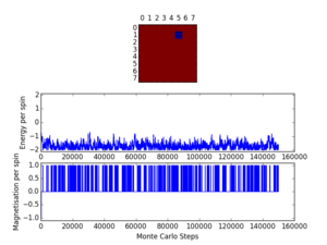
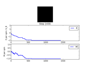
Using the presented script and the ILanim.py script, the Monte Carlo cycles can be simulated to view the results on the spin array as the process progresses. Here, the system under consideration was an 8 x 8 spin array, at a temperature of 0.5. Figure 3 shows the typical outcome of the animation, with the system having reached the most stable, minimum energy arrangement. For the result presented here, the output of the statistics() function was that shown in Table 3.

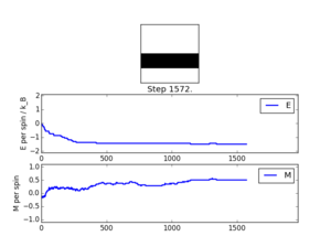
It was also observed that the system could locate a meta-stable state, with large regions of spin 'up' and 'down' spins. An example of such a result is presented in Figure 4 (for which the output data from statistics() is presented in Table 4).

NJ: well presented. Highlighting one of the metastable states is a nice touch.

Accelerating the code

In order to examine the efficiency of the python script developed thus far, the Iltimetrial.py script was utilised to investigate the time taken to perform 2000 Monte Carlo cycles. This script was modified to the version presented here, which repeats the time measurement a defined number of times, then calculates the average time and the standard error in this average. For the Monte Carlo script prepared previously, the average time for 2000 Monte Carlo cycles was measured to be 5.475804 s and a standard error was calculated to be 0.008325 s, with 100 measurements made using the script.

Evidently, the current script is slow at conducting large numbers of Monte Carlo cycles and hence, a more efficient script was developed using the np.roll, np.multiply and np.sum functions - this is presented here.

After this optimisation of the python script, the Iltimetrial.py script was re-run, giving an average time of 0.291467 s, with a standard error of 0.000156 s. Clearly, this optimised script is substantially faster than that developed previously (approximately 19 times faster).

NJ: are you surprised by what a difference this makes?

The effect of temperature

Correcting the averaging code

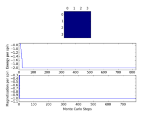
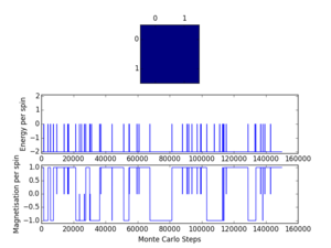
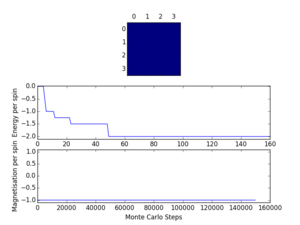
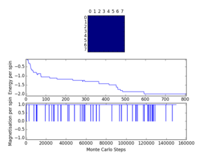
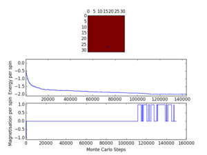
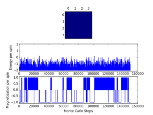
As the equilibrium state of the system requires a number of Monte Carlo cycles to be reached, it is evident that the average energies and magnetisations are accounting for values for non-equilibrium arrangements - this was accounted for through a consideration of the number of cycles required to reach equilibrium. For this, the ILfinalframe.py script was used, giving the graphs shown in Table 5. Here, each system was run for 150000 Monte Carlo cycles.

*Table 5: Graphs of energy and magnetisation versus number of Monte Carlo cycles for different temperatures and system sizes*
Temperature	System Size	Cycles for Equilibrium
0.5	4x4	24
0.5	8x8	392
0.5	16x16	5549
1.0	2x2	(0)
1.0	4x4	49
1.0	8x8	590
1.0	16x16	~6300
1.0	32x32	~110000
2.0	4x4	-
2.0	8x8	-

*Table 6: Number of cycles to be ignored for each system size*
System Size	Number of cycles before averaging
2x2	0
4x4	100
8x8	1000
16x16	8000
32x32	120000

Analysis of these graphs indicates that at higher temperatures, such as 2.0 (also observed at 1.5), large fluctuations in the energy and magnetisation are observed - these fluctuations are the reason that the average values of the properties must be taken. As the temperature is increased for systems of size 4x4, 8x8 and 16x16, it is clear that the number of cycles required in order to reach equilibrium increases. Hence, for the temperature range to be considered later (0.25 to 5.00), the required number of cycles was overestimated in order to ensure that all measurements were taken whilst the system was in equilibrium. The proposed numbers of cycles to be ignored for each system size are presented in Table 6.

NJ: there are bigger fluctuations at higher T, but the equilibration time decreases.

The python script developed up to this point was modified to account for these values by inclusion of a skip_region variable, which defines the number of cycles performed before energies and magnetisations contribute to the self.X values (before averaging occurs). The modified script is presented here.

Running over a range of temperatures

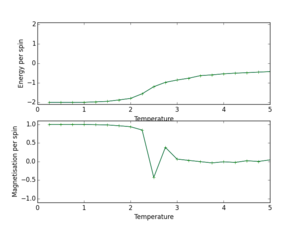
**Figure 5**: Average energy and average magnetisation vs. temperature for 8x8 lattice, with error bars

Using the python script modified in the previous exercise, the code can now be used to simulate the 8x8 system at a range of temperatures, using the ILtemperaturerange.py file (shown here). Here, the temperature range of 0.25 to 5.00 was used, with a separation of 0.25 between points, whilst the runtime was set to 10000 (neglecting the property values for the first 1000 cycles). Running this simulation produced the graphs in Figure 5, where error bars computed using standard errors have also been included (these are small as a consequence of small standard errors). From the graph of average energy versus temperature, the phase transition can be observed - this occurs in the region with a gradient that is not close to zero. The data used here (temperature, average energies, average squared-energies, average magnetisations and average squared-magnetisations) was then saved as a numpy array in a new file, 8x8.dat.

The effect of system size

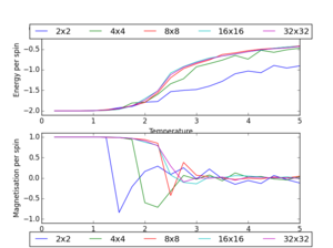
**Figure 6**: Average energy and average magnetisation (per spins) vs. temperature for multiple lattice sizes

The process conducted for the 8x8 lattice in the previous exercise was then repeated for lattices of sizes 2x2, 4x4, 16x16 and 32x32, with the data saved in .dat files. These files were then accessed, and the average energy and magnetisation data were plotted on one graph for all of the lattices sizes - this was achieved using the script presented here. The graphs produced in this manner are shown in Figure 6.

A consideration of this graph suggests that in order to capture the long range fluctuations, whilst minimising the computational time required, an 8x8 lattice is likely to be the optimum choice. This is because the graph for this system size is comparable to that for a 32x32 lattice, whilst being faster to compute.

NJ: nice presentation of the legend.

Determining the heat capacity

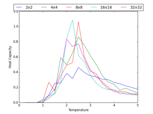
**Figure 7**: Heat capacity (per spin) versus temperature for different lattice sizes

Using the .dat files previously produced, the heat capacity was calculated for each lattice size using the equation

C = \frac{\partial E}{\partial T} = \frac{V a r [E]}{k_{B} T^{2}}

, (eq. 9)

where $V a r [E] = < E^{2} > - < E >^{2}$ . When implementing this, the k_B term was neglected due to the energy values having units of k_B. The script used for this purpose is provided here. The plot of heat capacity per spin versus temperature for all of the lattice sizes considered is presented in Figure 7.

Locating the Curie temperature

Comparison with C++ Data

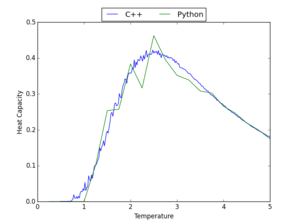
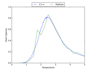
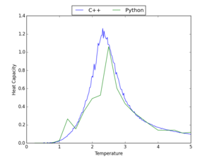
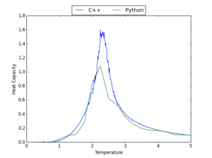
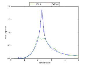
The data for the heat capacity generated using the python script prepared in this experiment was compared to that from longer C++ computations - graphs showing this comparison are presented in Table 7 for a range of lattice sizes. The Python code used to produce these graphs is shown here.

Considering these graphs, it is clear that, in general, there is a reasonable correlation between the Python and C++ data; however, some of the data, particularly that for high lattice sizes, shows that the Python computations have not always found the maximum of heat capacity. This correlation would be improved by making computations at the same range of temperatures, but with a smaller gap between the temperatures taken; however, this would substantially increase computation time.

NJ: and also increasing the number of MC cycles. The C++ code used 20,000 flips *per spin*.

*Table 7: Graphs of heat capacity (per spin) versus temperature for C++ and Python data*

2x2	4x4	8x8

16x16	32x32

Polynomial Fitting

**Figure 8**: Heat capacity (per spin) versus temperature for 8x8 system with two polynomial fits

In order to make use of the C++ data in finding the Curie temperature for the Ising Lattices under consideration, polynomials were fit to the data - the script written for this purpose is shown here. For this fitting, it was found that a polynomial order of 5 was required to provide a good fit for the 2x2 data - this increased significantly as the lattice size increased. An example fit is shown for the 8x8 system in Figure 8, where the polynomial fit is shown for orders 5 and 13. A consideration of this graph reveals that whilst a polynomial of order 5 may be appropriate for a 2x2 system, it is inadequate for the larger system of 8x8. Whilst an order of 13 substantially improves the polynomial fit, one must, in general, take care with 'overfitting' data.

NJ: you should be okay here, because there are lots of points, but this could be an issue. Mostly because this function isn't really a polymomial, and it gets less so as the number of spins increases

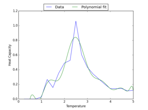
**Figure 9**: Heat capacity (per spin) versus temperature for Python data for 8x8 system with a 13th order polynomial fit

For comparison, a 13th order polynomial was fitted to the 8x8 Python data previously computed - this is shown in Figure 9. Here, it is evident that for this data, a higher order polynomial is required to obtain a fit comparable to that for the C++ data above.

Fitting in a Particular Temperature Range

**Figure 10**: Heat capacity (per spin) versus temperature for 8x8 system with peak polynomial fit

As was observed in the previous exercise, large polynomial orders are required to fit the C++ data well across the whole temperature range. The python script was modified to that presented here (this script also contains the python code to compute the maximum heat capacity and temperature at which this occurs for the following exercise), which fits a polynomial only in the region of the maximum heat capacity for the system. An example of such fit is shown in Figure 10 for the 8x8 system. Here, it should be noted that for all of the system sizes studied, a polynomial order of 3 was used - this is a clear improvement compared to the 13th order polynomials used previously.

Finding the Peak in Heat Capacity

*Table 8: Lattice sizes and their corresponding Curie temperatures*
System Size	Curie Temperature
2x2	2.53503504
4x4	2.43843844
8x8	2.33433433
16x16	2.30455455
32x32	2.27752753

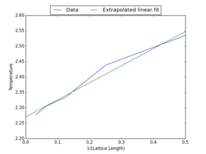
**Figure 11**: Curie temperature vs. 1/(lattice length), with extrapolated linear fit

In order to find the Curie temperature for an infinite Ising Lattice, the Curie temperature for each system size considered was first found (using the script shown in the previous exercise). These temperatures were then saved to a .dat file (whose contents are also showed in Table 8, along with their corresponding lattice sizes. Finally, using the script presented here, a graph of Curie temperature versus the inverse of the lattice length was plotted, according to the equation

T_{C, L} = \frac{A}{L} + T_{C, \infty}

, (eq. 10)

where $T_{C, L}$ is the Curie temperature for a lattice with length L and $T_{C, \infty}$ is the Curie temperature for an infinite Ising lattice. Hence, it is clear that the desired Curie temperature must be the y-intercept of the graph shown in Figure 11 (hence the use of extrapolation in the python script). Taking this extrapolated value gives a Curie temperature of 2.271. This value can be compared to the theoretical exact value of 2.27 (J/k_B),^[1] which indicates a good agreement between the value calculated in this investigation and the theoretical exact value. This is surprising given that it would be expected that the polynomial fitting of the data to locate the maximum would contribute a considerable degree of error to the final value. Alongside this, some error may also have been derived from the decision of the number of Monte Carlo cycles at which to begin averaging. In order to prevent any issues arriving here, a large number of cycles should be used - this was not implemented here due to the computation time that would be required.

NJ: careful. You've quoted your Curie temperature as 2.271, so you should quote the literature one to the same precision - 2.269. Good otherwise. The best thing you could do to improve the results is probably to simulate larger lattices and ignore the results from the small ones.

References

↑ D. K. Khudier, N. I. Fawaz, Int. Lett. Chem. Phys. Astron., 2013, 10, 201-212. Available from: http://www.ilcpa.pl/wp-content/uploads/2012/11/ILCPA-102-2013-201-2121.pdf

[1] D. K. Khudier, N. I. Fawaz, Int. Lett. Chem. Phys. Astron., 2013, 10, 201-212. Available from: http://www.ilcpa.pl/wp-content/uploads/2012/11/ILCPA-102-2013-201-2121.pdf

[1]