Talk:Mod:CMPpp2814

JC: General comments: All task answered, but with a few mistakes and some detail missing. Make sure your answers are clear to show that you understand the theory behind the tasks in this experiment and the significance of your results.

Introduction to the Ising Model

TASK: Show that the lowest possible energy for the Ising model is $E = - D N J$ , where D is the number of dimensions and N is the total number of spins. What is the multiplicity of this state? Calculate its entropy. Taking $E = - 1 / 2 J \sum_{i}^{N} \sum_{j} s_{i} s_{j}$ where j is the immediate neighbor of the spin in question i, and N is the total number of spins. The lowest possible energy requires that all of the spins be aligned- take spin +1, this makes the equation $E = 1 / 2 J N \sum_{j} s_{j}$ . Then look at the number of adjacent spins in 1D, 2D, and 3D lattices- for 1D there are 2, for 2D there are 4, and 3D there are 6. Therefore $\sum_{j} s_{j}$ is two times the number of dimensions D, giving the final result of $E = - D N J$ . From this you can calculate the energy using $S = k_{B} l n (w)$ . The multiplicity W is 2, as there are two possible configurations- all spin-up or all spin-down. Therefore the calculated entropy is 9.57 x 10^-24 J K^-1, which is very low. This makes sense, as a system with all of the spins aligned will be very ordered and hence have low entropy.

JC: Correct.

TASK: Imagine that the system is in the lowest energy configuration. To move to a different state, one of the spins must spontaneously change direction ("flip"). What is the change in energy if this happens (D=3, N=1000)? How much entropy does the system gain by doing so?

When the single spin flips, the general equation for energy must be used- $E = - 1 / 2 J \sum_{i}^{N} \sum_{j} s_{i} s_{j}$ . N=1000 and D=3. Then you have to consider not only the energy lost as a spin-up site is removed, but also the energy penalty of introducing a spin-down in that lattice site. This means there is the loss of 2x 2D for each dimension , which is less negative than the ground state energy, which makes sense, since the energy will be higher. The multiplicity W= N!/Л N_i= 1000, as the spin can be placed in any of the 1000 "lattice boxes" Hence the entropy is 9.53 x 10 ^-23, which means the entropy difference from the ground state is 8.57 x 10^-23.

JC: This is very unclear. The multiplicity for the single spin flipped case should be 2000 as you can have 1 spin down and all others up, or 1 spin up and all others down and there are 1000 spins.

TASK: Calculate the magnetisation of the 1D and 2D lattices in figure 1. What magnetisation would you expect to observe for an Ising lattice with D = 3, N=1000 at absolute zero?

For both of the 1D and 2D lattices, M=1, as for the 1D lattice, there are 3 spins of +1 and 2 spins of -1. For the 2D lattice there are 13 spins of +1 and 12 of -1. For the 3D Ising lattice with N=1000 at 0K would have a magnetization of (+/-)1000, as all of the spins would be aligned in the same spin state with no thermal energy to flip the spins.

JC: Correct.

Calculating the energy and magnetisation

TASK: complete the functions energy() and magnetisation(), which should return the energy of the lattice and the total magnetisation, respectively. In the energy() function you may assume that J=1.0 at all times (in fact, we are working in reduced units in which J=k_B, but there will be more information about this in later sections). Do not worry about the efficiency of the code at the moment — we will address the speed in a later part of the experiment.

The magnetisation function was

def magnetisation(self):
        "Return the total magnetisation of the current lattice configuration."
        magnetisation=0
        for spin in self.lattice:
            for i in spin:
                magnetisation=magnetisation + i
        return magnetisation

The energy function was:

def energy(self):
        "Return the total energy of the current lattice configuration."
        constant=0.5
        energy=0

        for i in range(self.n_rows):
            for j in range(self.n_cols):
        
                 row = i
                 column = j
        
                 if row == 0:
                     if column == 0:
                         interaction1=self.lattice[0,0]*self.lattice[0,-1]
                         interaction2=self.lattice[0,0]*self.lattice[-1,0]
                         interaction3=self.lattice[0,0]*self.lattice[0,1]
                         interaction4=self.lattice[0,0]*self.lattice[1,0]
                         energy=energy+interaction1+interaction2+interaction3+interaction4
            
                     elif column == self.n_cols - 1:
                         interaction_one=self.lattice[0,self.n_cols-1]*self.lattice[0,0]
                         interaction_two=self.lattice[0,self.n_cols-1]*self.lattice[self.n_rows-1, self.n_cols-1]
                         interaction_three=self.lattice[0,self.n_cols-1]*self.lattice[0,self.n_cols-2]
                         interaction_four=self.lattice[0,self.n_cols-1]*self.lattice[1,self.n_cols-1]
                         energy=energy+interaction_one+interaction_two+interaction_three+interaction_four
            
                     else:
                         interaction_1=self.lattice[0,column]*self.lattice[-1,column]
                         interaction_2=self.lattice[0,column]*self.lattice[0, column-1]
                         interaction_3=self.lattice[0,column]*self.lattice[0, column+1]
                         interaction_4=self.lattice[0,column]*self.lattice[1,column]
                         energy=energy+interaction_1+interaction_2+interaction_3+interaction_4
                
                 elif row == self.n_rows-1:
                     if column==0:
                         inter_1=self.lattice[self.n_rows-1,0]*self.lattice[self.n_rows-1, -1]
                         inter_2=self.lattice[self.n_rows-1,0]*self.lattice[0,0]
                         inter_3=self.lattice[self.n_rows-1,0]*self.lattice[self.n_rows-1,1]
                         inter_4=self.lattice[self.n_rows-1,0]*self.lattice[self.n_rows-2,0]
                         energy=energy+inter_1+inter_2+inter_3+inter_4
                
                     elif column== self.n_cols-1:
                         inter_one=self.lattice[self.n_rows-1,self.n_cols-1]*self.lattice[self.n_rows-1,0]
                         inter_two=self.lattice[self.n_rows-1,self.n_cols-1]*self.lattice[0,self.n_cols-1]
                         inter_three=self.lattice[self.n_rows-1, self.n_cols-1]*self.lattice[self.n_rows-1,self.n_cols-2]
                         inter_four=self.lattice[self.n_rows-1,self.n_cols-1]*self.lattice[self.n_rows-2,self.n_cols-1]
                         energy=energy+inter_one+inter_two+inter_three+inter_four
                
                     else:
                         inter1=self.lattice[self.n_rows-1, column]*self.lattice[self.n_rows-1,column-1]
                         inter2=self.lattice[self.n_rows-1, column]*self.lattice[0,column]
                         inter3=self.lattice[self.n_rows-1, column]*self.lattice[self.n_rows-1,column+1]
                         inter4=self.lattice[self.n_rows-1, column]*self.lattice[self.n_rows-2,column]
                         energy=energy+inter1+inter2+inter3+inter4

                 elif column == 0:
                    one=self.lattice[row,0]*self.lattice[row,-1]
                    two=self.lattice[row,0]*self.lattice[row, 1]
                    three=self.lattice[row,0]*self.lattice[row-1,0]
                    four=self.lattice[row,0]*self.lattice[row+1, 0]
                    energy=energy+one+two+three+four
            
                 elif column == self.n_cols-1:
                    uno=self.lattice[row,self.n_cols-1]*self.lattice[row,0]
                    dos=self.lattice[row,self.n_cols-1]*self.lattice[row, self.n_cols-2]
                    tres=self.lattice[row,self.n_cols-1]*self.lattice[row-1,self.n_cols-1]
                    quatro=self.lattice[row,self.n_cols-1]*self.lattice[row+1, self.n_cols-1]
                    energy=energy+uno+dos+tres+quatro

                 else:
                     action1=self.lattice[row,column]*self.lattice[row-1,column]
                     action2=self.lattice[row, column]*self.lattice[row+1, column]
                     action3=self.lattice[row, column]*self.lattice[row, column-1]
                     action4=self.lattice[row, column]*self.lattice[row, column+1]
                     energy=energy+action1+action2+action3+action4

            final_energy= -1 * constant * energy  
            
        return final_energy

JC: Code looks correct, but you should include comments to make it easier to read and try to simplify it a bit, there is no need to include different names for the interactions, e.g. interaction1, interaction_one, interaction_1 etc.

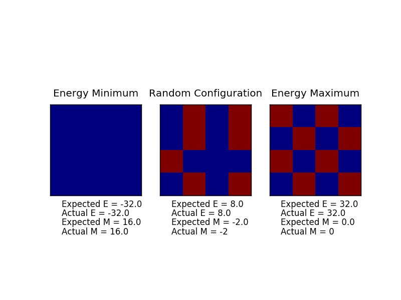
TASK: Run the ILcheck.py script from the IPython Qt console using the command

Figure 1: ILcheck.py output to show that the code works.

Introduction to the Monte Carlo simulation

TASK: How many configurations are available to a system with 100 spins? To evaluate these expressions, we have to calculate the energy and magnetisation for each of these configurations, then perform the sum. Let's be very, very, generous, and say that we can analyse 1\times 10^9 configurations per second with our computer. How long will it take to evaluate a single value of \left\langle M\right\rangle_T?

There are 2^100 possible configurations. With that computational power it would take 1.27 x 10^21 seconds, which is 4.02 x 10^13 years. Way too long!

TASK: Implement a single cycle of the above algorithm in the montecarlocycle(T) function. This function should return the energy of your lattice and the magnetisation at the end of the cycle. You may assume that the energy returned by your energy() function is in units of k_B! Complete the statistics() function. This should return the following quantities whenever it is called: <E>, <E^2>, <M>, <M^2>, and the number of Monte Carlo steps that have elapsed.

def montecarlostep(self, T):
        # complete this function so that it performs a single Monte Carlo step
        initial=np.copy(self.lattice)
        initialE=self.energy()
        #the following two lines will select the coordinates of the random spin for you
        random_i = np.random.choice(range(0, self.n_rows))
        random_j = np.random.choice(range(0, self.n_cols))
        #the following line will choose a random number in the rang e[0,1) for you
        random_number = np.random.random()
        #the following line creates the new lattice with one flipped spin
        self.lattice[random_i, random_j]=self.lattice[random_i, random_j] * -1
        energy = self.energy()
        magnetisation=self.magnetisation()
        delta_E= energy-initialE

        if delta_E < 0:
            self.E=self.E+energy
            self.M= self.M+magnetisation
            self.E2=self.E2+energy**2
            self.M2=self.M2+magnetisation**2
            
            
        elif delta_E >= 0:
            boltzy=math.exp(-delta_E/T)
            #the key part of the Monte Carlo method- remember units are in kB!
            if random_number <= boltzy:
                self.E=self.E+energy
                self.M= self.M+magnetisation
                self.E2=self.E2+energy**2
                self.M2=self.M2+magnetisation**2
                
                
            else:
                #disregard if the random number is greater than bolzy
                self.lattice=initial
              
        self.n_cycles=self.n_cycles+1

def statistics(self):
        # complete this function so that it calculates the correct values for the averages of E, E*E (E2), M, M*M (M2), and returns the
        av_e=self.E/self.n_cycles 
        av_e2=self.E2/self.n_cycles
        av_m=self.M/self.n_cycles
        av_m2=self.M2/self.n_cycles
        return av_e, av_e2, av_m, av_m2

TASK: If T < T_C, do you expect a spontaneous magnetisation (i.e. do you expect $⟨ M ⟩ \neq 0)$ ? When the state of the simulation appears to stop changing (when you have reached an equilibrium state), use the controls to export the output to PNG and attach this to your report. You should also include the output from your statistics() function.

Since the temperature is below the critical temperature (or Curie temperature), I would expect spontaneous magnetisation, as there is not yet enough thermal energy to destroy the ordering of the spins. This is supported by the simulation output- after a certain number of cycles (which varies from lattice size to lattice size and temperature to temperature), a system with overwhelmingly more of one spin is produced. Here you can see the simple 8x8 lattice at temperature 1.0. It reaches a stable equilibrium of all-aligned spins in fairly few steps.

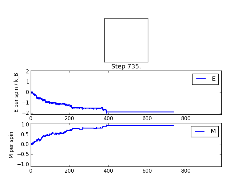
Figure 2: ILanim.py output showing spontaneous magnetisation

Averaged quantities: E = -1.7375 E*E = 3.21944901316 M = 0.882072368421 M*M = 0.825251850329

Accelerating the Code

TASK: Use the script ILtimetrial.py to record how long your current version of IsingLattice.py takes to perform 2000 Monte Carlo steps. This will vary, depending on what else the computer happens to be doing, so perform repeats and report the error in your average!

My current version takes on average 11.113s to run, with a standard deviation of 0.171s.

JC: How many simulations did you use to calculate this average and standard deviation?

TASK: Look at the documentation for the NumPy sum function. You should be able to modify your magnetisation() function so that it uses this to evaluate M. The energy is a little trickier. Familiarise yourself with the NumPy roll and multiply functions, and use these to replace your energy double loop (you will need to call roll and multiply twice!). The magnetisation simply requires the sum function twice:

def magnetisation(self):
        "Return the total magnetisation of the current lattice configuration."
        return sum(sum(self.lattice))

To deal with the energy is more complicated, due to the difference in logic between the code that I have written and how roll is meant to be used.

        roll_1=np.roll(self.lattice,1, 1)
        roll_3=np.roll(self.lattice,1,0)
        one=np.multiply(self.lattice, roll_1)
        three=np.multiply(self.lattice, roll_3)
        summat=one+three
        almost_there=sum(sum(summat))
        final_energy=-1*almost_there
        return final_energy

Only two shifts were needed, as this accounts for all of the spin interactions- accordingly the factor of a half was removed, as that accounted for double-counting interactions.

JC: Well noticed that you only need to use roll twice.

TASK: Use the script ILtimetrial.py to record how long your new version of IsingLattice.py takes to perform 2000 Monte Carlo steps. This will vary, depending on what else the computer happens to be doing, so perform repeats and report the error in your average!

The new version takes on average 0.514s to take 2000 monte carlo steps, with a standard deviation of 0.014s. This is a lot faster (and more consistent with the time taken), requiring less computing power and time. Definitely a bonus!

The effect of temperature

TASK: The script ILfinalframe.py runs for a given number of cycles at a given temperature, then plots a depiction of the final lattice state as well as graphs of the energy and magnetisation as a function of cycle number. This is much quicker than animating every frame! Experiment with different temperature and lattice sizes. How many cycles are typically needed for the system to go from its random starting position to the equilibrium state? Modify your statistics() and montecarlostep() functions so that the first N cycles of the simulation are ignored when calculating the averages. You should state in your report what period you chose to ignore, and include graphs from ILfinalframe.py to illustrate your motivation in choosing this figure.

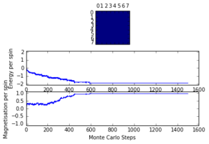
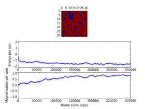
For a 8x8 lattice at a temperature of 1.0, as can be seen my Figure #, the equilibrium is reached quite quickly, at less than 1000 steps. However, as the lattice size and temperature both increase, the time taken for equilibrium to be reached increases quite a bit. At a temperature of 2.2 (close to the critical temperature, can be told from the magnetisation/timerange graph) there is still quite a bit of fluctuation around step 100 000. In order to ensure that the equilibrium was reached for the largest and warmest systems, the number of cycles to ignore was set at 150 000.

Modified montecarlostep() and statistics() functions:

if delta_E < 0:
            if self.n_cycles >150000:
                
                self.E=self.E+energy
                self.M= self.M+magnetisation
                self.E2=self.E2+energy**2
                self.M2=self.M2+magnetisation**2
            
            
        elif delta_E >= 0:
            boltzy=math.exp(-delta_E/T)
            #the key part of the Monte Carlo method- remember units are in kB!
            if random_number <= boltzy:
                if self.n_cycles >150000:
                    self.E=self.E+energy
                    self.M= self.M+magnetisation
                    self.E2=self.E2+energy**2
                    self.M2=self.M2+magnetisation**2
                
                
            else:
                #disregard if the random number is greater than bolzy
                if self.n_cycles >150000:
                    self.E=self.E+initialE
                    self.M= self.M+initialM
                    self.E2=self.E2+initialE**2
                    self.M2=self.M2+initialM**2
                self.lattice=initial

av_e=self.E/(self.n_cycles -150000)
        av_e2=self.E2/(self.n_cycles-150000)
        av_m=self.M/(self.n_cycles-150000)
        av_m2=self.M2/(self.n_cycles-150000)

The number of cycles to ignore was accounted for in the monte carlo method by putting if statements in front of anything that added to the energy and magnetisation values. In the statistics, this was included to ensure that accurate averages were calculated by subtracting the 150 000 from the n_cycles that were not counted.

JC: Check the formatting of your code, are the indents correct here? You could have made the number of steps to ignore a variable so that it could be easily changed throughout your code. How long does it take to reach equilibrium above the Curie temperature?

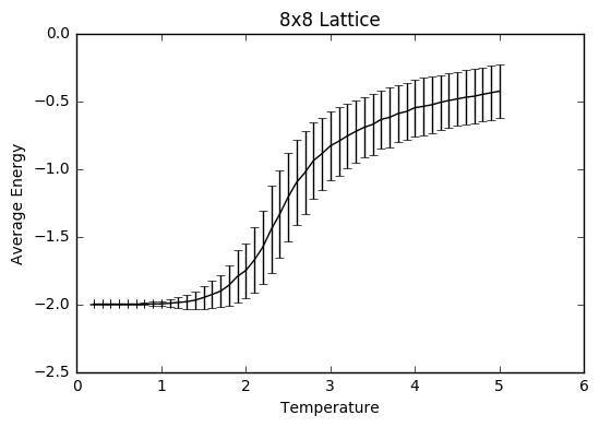
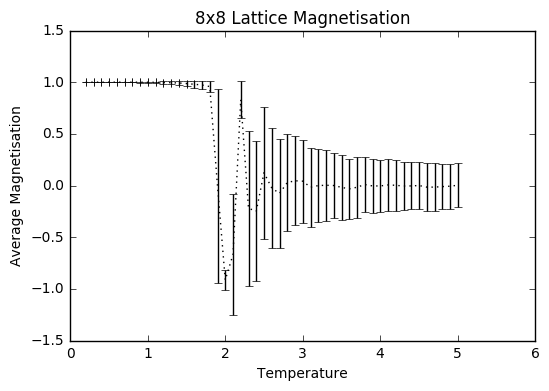
TASK: Use ILtemperaturerange.py to plot the average energy and magnetisation for each temperature, with error bars, for an 8\times 8 lattice. Use your initution and results from the script ILfinalframe.py to estimate how many cycles each simulation should be. The temperature range 0.25 to 5.0 is sufficient. Use as many temperature points as you feel necessary to illustrate the trend, but do not use a temperature spacing larger than 0.5. T NumPy function savetxt() stores your array of output data on disk — you will need it later. Save the file as 8x8.dat so that you know which lattice size it came from

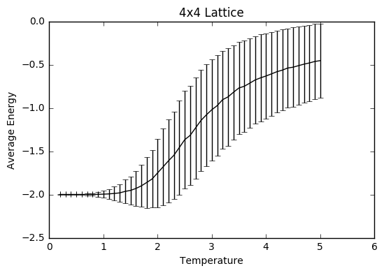
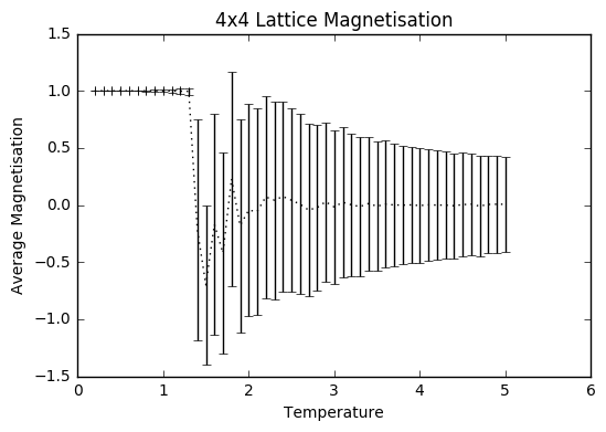
The temperature range was selected to be 0.2-5 with steps of 0.1 to save time and sanity, so the computations only took 35-40 minutes each. The number of simulations was set to be 400 000, to ensure that there was a large enough sample size after the equilibrating steps that were discarded to give a more accurate average, taking into account all the the fluctuations, especially the ones at higher temperatures.

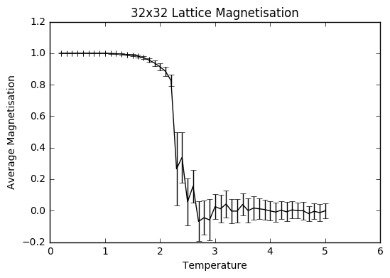
As can be seen from the graphs, the average energy at temperature 1.0 is more negative than the average values from the ILanim.py file, which shows that the beginning part where the system is still equilibrating has been removed. The trend of increasing error bar size makes sense: as the temperature goes up, the variation goes up due to the greater thermal energy present.

JC: Why are the error bars largest around the Curie temperature?

The code used to plot these graphs (and a variation later used to plot the graphs of different size):

eight_data=np.loadtxt('_8x8_one.dat')

temp8=eight_data[:,0]
av_E8=eight_data[:,1]
av_E28=eight_data[:,2]
av_M8=eight_data[:,3]
av_M28=eight_data[:,4]
diff8=av_E28-(av_E8**2)
error8=np.sqrt(abs(diff8))/64

plt.errorbar(temp8, av_E8/64, xerr=0, yerr=error8, ls='solid', color='black')
plt.ylabel('Average Energy')
plt.xlabel("Temperature")
plt.title("8x8 Lattice")
plt.show()

diff8m=av_M28-(av_M8**2)
error8M=np.sqrt(abs(diff8m))/64

plt.errorbar(temp8, av_M8/64, xerr=0, yerr=error8M, ls='solid', color='black')
plt.ylabel('Average Magnetisation')
plt.xlabel("Temperature")
plt.title("8x8 Lattice Magnetisation")
plt.show()

The effect of system size

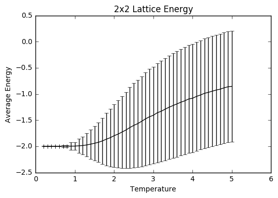
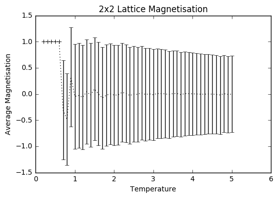
TASK: Repeat the final task of the previous section for the following lattice sizes: 2x2, 4x4, 8x8, 16x16, 32x32. Make sure that you name each datafile that your produce after the corresponding lattice size! Write a Python script to make a plot showing the energy per spin versus temperature for each of your lattice sizes. Hint: the NumPy loadtxt function is the reverse of the savetxt function, and can be used to read your previously saved files into the script. Repeat this for the magnetisation. As before, use the plot controls to save your a PNG image of your plot and attach this to the report. How big a lattice do you think is big enough to capture the long range fluctuations?

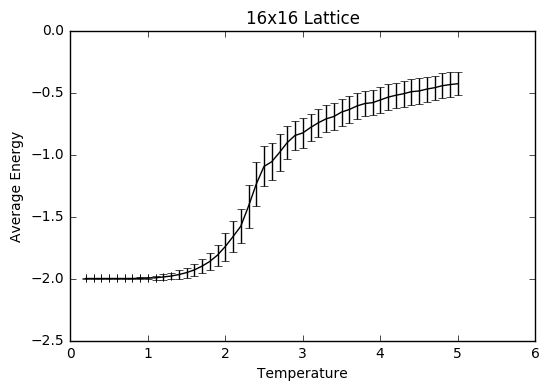
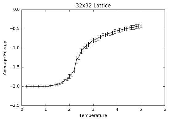
The settings were: N=150 000 to take into account larger lattice sizes and higher temperatures requiring longer for the equilibrium temperature to be reached. The total number of steps in the temperaturerange is 400 000 to ensure a nice large sample size. The range of temperatures is between 0.2 and 5 (including), increasing by steps of 0.1 to ensure moderate accuracy and to ensure that the computations could be completed within a semi-reasonable time frame.

The variance decreases with increasing lattice size probably due to the increased number of sample spins. As the boltzmann distribution is meant for larger systems, the calculations only become more accurate with larger systems, meaning that one state dominates. Hence, as one state becomes more and more dominant, the variation decreases.

Determining the heat capacity

TASK: By definition,

$C = \frac{\partial ⟨ E ⟩}{\partial T}$

From this, show that

$C = \frac{V a r [E]}{k_{B} T^{2}}$

(Where $V a r [E]$ is the variance in E.)

Using this relation, and the data that you generated in the previous sections, you can now determine the heat capacity of your lattice as a function of temperature and system size.

In order to show this relation, the expression for average energy must be expressed in terms of the partition function $Q = \sum_{i} \exp (\frac{- E_{i}}{k_{B} T})$ ^[1]

$⟨ E ⟩ = \frac{\sum_{i} E_{i} \exp (\frac{- E_{i}}{k_{B} T})}{\sum_{i} \exp (\frac{- E_{i}}{k_{B} T}})$

$C_{v} = \frac{\partial}{\partial T} \frac{\sum_{i} E_{i} \exp (\frac{- E_{i}}{k_{B} T})}{\sum_{i} \exp (\frac{- E_{i}}{k_{B} T}})$

This needs to be differentiated using the quotient and chain rule:

$C_{v} = \frac{\frac{\partial}{\partial T} \sum_{i} E_{i} \exp (\frac{- E_{i}}{k_{B} T})}{\sum_{i} \exp (\frac{- E_{i}}{k_{B} T})} - \frac{\sum_{i} E_{i} \exp (\frac{- E_{i}}{k_{B} T})}{\sum_{i} \exp (\frac{- E_{i}}{k_{B} T})^{2}} * \frac{\partial}{\partial T} (\sum_{i} \exp (\frac{- E_{i}}{k_{B} T}))$

$C_{v} = \frac{\sum_{i} \frac{E_{i}^{2}}{k_{B} T} \exp (\frac{- E_{i}}{k_{B} T})}{\sum_{i} \exp (\frac{- E_{i}}{k_{B} T})} - \frac{\sum_{i} E_{i} \exp (\frac{- E_{i}}{k_{B} T})}{\sum_{i} \exp (\frac{- E_{i}}{k_{B} T})^{2}} * (\sum_{i} \frac{E_{i}^{2}}{k_{B} T} \exp (\frac{- E_{i}}{k_{B} T})$

$C_{v} = \frac{1}{k_{B} T^{2}} (\frac{\sum_{i} E_{i}^{2} \exp (\frac{- E_{i}}{k_{B} T})}{\sum_{i} \exp (\frac{- E_{i}}{k_{B} T})} - (\frac{\sum_{i} E_{i} \exp (\frac{- E_{i}}{k_{B} T})}{\sum_{i} \exp (\frac{- E_{i}}{k_{B} T})})^{2}$

The first half of that expression is equivalent to $⟨ E^{2} ⟩$ , the second half is equivalent to ${⟨ E ⟩}^{2}$ Hence you get

 $C_{v} = \frac{⟨ E^{2} ⟩ - {⟨ E ⟩}^{2}}{k_{B} T^{2}} = \frac{V a r [E]}{k_{B} T^{2}}$

JC: Good derivations, but a few typos between steps like the factor of E^2/kT^2 in the first term.

TASK: Write a Python script to make a plot showing the heat capacity versus temperature for each of your lattice sizes from the previous section. You may need to do some research to recall the connection between the variance of a variable, $V a r [X]$ , the mean of its square $⟨ X^{2} ⟩$ , and its squared mean ${⟨ X ⟩}^{2}$ . You may find that the data around the peak is very noisy — this is normal, and is a result of being in the critical region. As before, use the plot controls to save your a PNG image of your plot and attach this to the report.

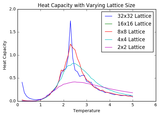
As can be seen in the figure, the shape of the heat capacity curve becomes much more peaked as the lattice size increases. There some amount of noise around the peak, however not as much as may be expected. This may be because I ran the simulation for a fairly long time beyond the time required for equilibration.. The peaks also shift as the lattice increases in size- this shows the impact of the finite size effect.

An example of the code used to generate the plot. First the data was extracted from the files in the method of the example below (used for lattice size 4):

tempfour=latticefour[:,0]
avEfour=latticefour[:,1]
avsquared=latticefour[:,2]
diffFour=avsquared-(avEfour**2)
CvFour=diffFour/(tempfour**2)

Then all of the data was plotted on the same graph to visualize how the heat capacity changes with lattice size.

#graph comparing them all
plotTemp32, = plt.plot(temp32,Cv32/1024, label = '32x32 Lattice')
plotTemp16, = plt.plot(temp16,Cv16/256, label = '16x16 Lattice')
plotTemp8, = plt.plot(temp8,Cv8/264, label = '8x8 Lattice')
plotTemp4, = plt.plot(tempfour,CvFour/16, label = '4x4 Lattice')
plotTemp2, = plt.plot(temptwo,Cvtwo/4, label = '2x2 Lattice')
plt.legend(handles=[plotTemp32, plotTemp16, plotTemp8, plotTemp4, plotTemp2])
plt.ylim(0,.2)
plt.ylabel('Heat Capacity')
plt.xlabel('Temperature')
plt.title('Heat Capacity with Varying Lattice Size')
plt.show()

Locating the Curie Temperature

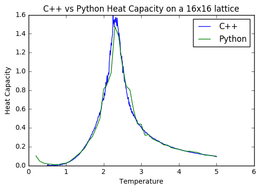
TASK: A C++ program has been used to run some much longer simulations than would be possible on the college computers in Python. You can view its source code here if you are interested. Each file contains six columns: T, E, E^2, M, M^2, C (the final five quantities are per spin), and you can read them with the NumPy loadtxt function as before. For each lattice size, plot the C++ data against your data. For one lattice size, save a PNG of this comparison and add it to your report — add a legend to the graph to label which is which. To do this, you will need to pass the label="..." keyword to the plot function, then call the legend() function of the axis object .

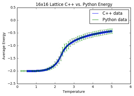
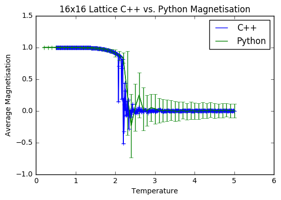
It is interesting to note that for the average energy and magnetisation from both computations, the data sets match quite well- the main difference is with the error bars; they are somewhat larger on the Python data. This is presumably because the method of that simulation is much less thorough, allowing for greater fluctuations. The heat capacities are also quite well matched, with the Python data showing less noise on a finer level, due to the fact that the temperature steps were comparatively large. I assume that this close match of the C++ data and my Python data is due to the fact that I excluded 150 000 steps to allow for a thorough equilibration, and then did a total of 400 000 steps to ensure a good sample size was achieved.

JC: Both data sets are generated using the same importance sampling Monte Carlo method, but the C++ data has been generated using a longer simulation.

The code written to plot these graphs is based on this code (for just the energy):

data_16=np.loadtxt("16x16.dat")
data16=np.loadtxt('_16x16_one.dat')

temp_16=data_16[:,0]
avE_16=data_16[:,1]
av_sq_16=data_16[:,2]

temp16=data16[:,0]
avE16=data16[:,1]
av_sq16=data16[:,2]

diff16=av_sq16-(avE16**2)
root16=np.sqrt(diff16)
var16=root16/(16**2)
diff_16=av_sq_16-(avE_16**2)
root_16=np.sqrt(abs(diff_16))
var_16=root_16/(16**2)

plt.errorbar(temp_16, avE_16, xerr=0, yerr=var_16, color='blue',marker=None)
plt.errorbar(temp16, avE16/256, xerr=0, yerr=var16, color='green', marker=None)
CPLUS,=plt.plot(temp_16, avE_16,label='C++ data')
PYTH,=plt.plot(temp16, avE16/256,label='Python data')
plt.legend(handles=[CPLUS,PYTH])
plt.ylim(-2.5, 0.5)
plt.ylabel('Average Energy')
plt.xlabel("Temperature")
plt.title("16x16 Lattice C++ vs. Python Energy")
plt.show()

TASK: write a script to read the data from a particular file, and plot C vs T, as well as a fitted polynomial. Try changing the degree of the polynomial to improve the fit — in general, it might be difficult to get a good fit! Attach a PNG of an example fit to your report.

The peak was fitted to the C++ file data, as that is presumably much more accurate than that obtained from the Python simulations.

This fit was achieved with a 5th order polynomial for the 2x2 lattice. For the 16x16 lattice, however, no matter how high the order of the polynomial, it could not be fitted to the sharp peak.

JC: What order polynomial did you try up to? A higher order polynomial should have given a better fit than this.

The code written to plot the graphs is (for the 2x2 lattice, but basically the same for the other lattice sizes):

For the fitting to the entire temperature range (example for the 2x2 lattice):

two=np.loadtxt('2x2.dat')

T2=two[:,0]
C2=two[:,5]

fit=np.polyfit(T2,C2,5)
T_min=np.min(T2)
T_max=np.max(T2)
T_range=np.linspace(T_min,T_max,1000)
fitted_C_values=np.polyval(fit,T_range)

cpls,=plt.plot(T2,C2, color='red',label='Heat Capacity')
pythy,=plt.plot(T_range,fitted_C_values, color='blue',label='Fitted Curve')
plt.legend(handles=[cpls,pythy], loc=4)
plt.title('2x2 Heat Capacity Curve Fitting')
plt.xlabel('Temperature')
plt.ylabel("Heat Capacity")
plt.show()

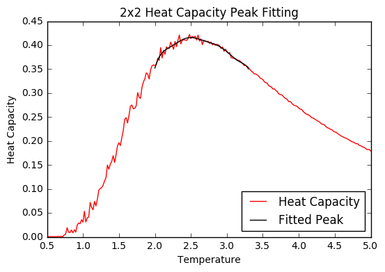
TASK: Modify your script from the previous section. You should still plot the whole temperature range, but fit the polynomial only to the peak of the heat capacity! You should find it easier to get a good fit when restricted to this region.

As the peak gets narrower, the worse the polynomial curve fits to the data points, and the more important it is to plot only to a narrow range of temperatures to get the max heat capacity and an accurate critical temperature value.

For fitting the restricted temperature range (again example for the 2x2 lattice):

t_min=2
t_max=3.3
t_range=np.linspace(t_min,t_max, 1000)
selection=np.logical_and(T2> t_min, T2 < t_max)
peak_T2=T2[selection]
peak_C2=C2[selection]
Fit=np.polyfit(peak_T2, peak_C2,10)
Fitted_C=np.polyval(Fit,t_range)

curve,=plt.plot(T2,C2, color='red',label='Heat Capacity')
thefit,=plt.plot(t_range,Fitted_C,color='black',label='Fitted Peak')
plt.legend(handles=[curve,thefit], loc=4)
plt.title('2x2 Heat Capacity Peak Fitting')
plt.ylabel('Heat Capacity')
plt.xlabel('Temperature')
plt.show()

JC: Fit to 2x2 data looks good, it would have been good to have included the other systems as well.

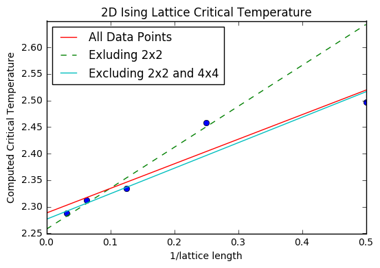
TASK: find the temperature at which the maximum in C occurs for each datafile that you were given. Make a text file containing two colums: the lattice side length (2,4,8, etc.), and the temperature at which C is a maximum. This is your estimate of T_C for that side length. Make a plot that uses the scaling relation given above to determine T_{C,\infty}. By doing a little research online, you should be able to find the theoretical exact Curie temperature for the infinite 2D Ising lattice. How does your value compare to this? Are you surprised by how good/bad the agreement is? Attach a PNG of this final graph to your report, and discuss briefly what you think the major sources of error are in your estimate.

Once the critical temperatures were extracted from the heat capacity data, they were plotted against 1/(lattice side length), in accordance to the scaling relation $T_{C, L} = \frac{A}{L} + T_{C, \infty}$ . The y intercept of the resulting line of best fit is the critical temperature for an infinite 2D Ising lattice.

The code for calculating the linear regression and plotting the graph:

from scipy import stats
slope, intercept, r_value, p_value, std_err=stats.linregress(lttc, ct)
slope1, intercept1, r_value1, p_value1, std_err1=stats.linregress(lattice_length, C_t)
slope2, intercept2, r_value2, p_value2, std_err2=stats.linregress(l, C)

x=np.linspace(0,0.5,1000)

plt.plot(lattice_length,C_t, ls='', marker="o")
almost,=plt.plot(x, slope*x + intercept,ls='--',label='Exluding 2x2')
al,= plt.plot(x, slope1*x +intercept1, label='All Data Points')
nearly,=plt.plot(x, slope2*x +intercept2, label='Excluding 2x2 and 4x4')
plt.legend(handles=[al,almost,nearly], loc=2)
plt.title('2D Ising Lattice Critical Temperature')
plt.xlabel('1/lattice length')
plt.ylabel('Computed Critical Temperature')
plt.show()

(Print statements were used to get the intercept from the linear regression calculation.)

Multiple lines of best fit were included. First, all of the critical temperatures were included in the linear regression calculation. This yielded T_infinity =2.288. However, due to the documented unreliability of the 2x2 lattice (the breadth of the peak), this was then excluded in the next linear regression calculation to find a second line of best fit. This yielded T_infinity =2.258. Finally, only the three data points with the largest lattice sizes were included, giving T_infinity =2.278. The literature value from an analytical treatment of the model is 2.269^[2].This is between the values of the second and third lines of best fit, indicating that the exclusion of the smaller lattice sizes improved the accuracy, but that only having 3 data points does not suffice for a thoroughly accurate line of best fit. So the major source of error (that was then negated) was the inclusion of a poor lattice model (2x2). If my python data had been used, some error would have come from the fact that the temperature steps were relatively large, at 0.1. Much smaller temperature steps could have been used, and more time allowed for the system to equilibrate, especially for the larger temperatures. A greater number of total steps could have been used, although overall the comparison of my results to the C++ data shows a pretty high degree of agreement. A greater error would be the fact that larger and more lattice sizes were not included- a 64x64 lattice size, or 128x128 would presumably have allowed for greater accuracy if also included.

Ultimately, the degree to which T_infinity was close to the analytical answer is astonishingly good, and shows that both methods have strong agreement, which speaks in favour of using both approaches. The combination of analytical and computational techniques is very powerful, but should an analytical result be too difficult to find, this shows that a computational approach can be just as good.

JC: Good.

References

↑ 2.J. Seddon and J. Gale, Thermodynamics and statistical mechanics, Royal Society of Chemistry, Cambridge, UK, 1st edn., 2001.
↑ 1.L. Onsager, Physical Review, 1944, 65, 117-149.

[1] 2.J. Seddon and J. Gale, Thermodynamics and statistical mechanics, Royal Society of Chemistry, Cambridge, UK, 1st edn., 2001.

[2] 1.L. Onsager, Physical Review, 1944, 65, 117-149.

[1]

[2]