Talk:Mod:CMPSimulations
NJ: General comments. Take a bit more care with your writing, there are a few sentences in the report that don't really make sense, as well as some minor spelling and grammar points. Your graphs are quite clear on the whole, but why did you not use the PNG image exporter more often?
The objective of the following computation is to derive energy and magnetisation outputs for any given lattice generated from Monte-Carlo simulations. The energetic and magnetic properties of the lattice are described by the Ising model, which relies on a collection of spins. Ising model describes ferromagnetic materials and using the simulations below, the heat capacity properties as well as second order phase transitions for ferromagnetic lattices can be derived.
Section 1: Introduction to the Ising Model
Key ideas included in this section include: a) Ising Model is a method to describe ferromagnetic materials based on energy minimisation and entropy maximisation. b) Demonstrated that for a lattice of dimension D, there are a total of 2D interactions and therefore the ground state energies can be simplified to be E = -DNJ. c) Calculated the changes in energy and magnetisation upon phase transitions.
TASK: Show that the lowest possible energy for the Ising model is E = -DNJ, where D is the number of dimensions and N is the total number of spins. What is the multiplicity of this state? Calculate its entropy.
The most energetically favorable arrangement involves parallel alignment of all magnetic moments. The spins are correlated to each other with respect to the energy in the following equation:

For any given lattice of any dimension, there are always a total of 2D interactions per cell, where D is the number of dimensions of the lattice. Therefore, the sum of Si and Sj spins interactions is equal to 2D (in 1D, there are 2 adjacent cells next to the specified cell, in 2D, there are 4 adjacent cells...).
This reduces the interaction energy equation to:
By observation of the interaction energy equation, the ground states occur when all spins have the same sign (ie. all +1 or -1). Therefore, the multiplicity for ground states, W = 2, is derived from a total of two microstates.

TASK: Imagine that the system is in the lowest energy configuration. To move to a different state, one of the spins must spontaneously change direction ("flip"). What is the change in energy if this happens (D=3, N=1000)? how much entropy does the system gain by doing so?
For a lattice system with 1000 cells in 3 dimensions, the interaction energy can be expressed as:
E = -0.5(2DNJ), where D refers to the number of dimensions, N as the number of cells in the lattice and J is an undefined constant. The process of flipping one spin incurs energetic penalty, such that there is a loss of favourable interactions between parallel spins and a gain of unfavourable interactions with antiparallel spins. Given that this is a three-dimensional lattice, there exists a total of six interactions for the particular cell with a flipped spin. As a result,
The energy of the new lattice is E = -0.5J(2DN - 6 - 6) = J(DN + 6) = +3006 J
The energy change incurred in the process of flipping a spin is therefore, ΔE = +6 J
NJ: Not quite. As well as gaining unfavourable interactions, you also lose favourable ones. The energy change is +12J.
As a spin flipping occurred, there must be a positive change in entropy, which is expressed below:
ΔS = kln(1000) - kln(2) = +8.58 x 10⁻²³ m2 kg s-2 K-1
NJ: The new multiplicity is 2000 - you have two choices of spin (up or down), and 1000 places to put that spin. Correct otherwise.
TASK: Calculate the magnetisation of the 1D and 2D lattices in figure 1. What magnetisation would you expect to observe for an Ising lattice with D = 3, N = 1000 at absolute zero?
The total magnetisation of the system is defined as:

For the 1D lattice, which has N = 5, the total magnetisation is +1.
For the 2D lattice, which has N = 25, the total magnetisation is +1.
At absolute zero, there is little thermal energy to overcome the required energy barrier to achieve random configurations. Therefore, the expected magnetisation at low temperatures should involve nearly uniform parallel spins, making the magnetisation per cell equal to +1 or -1 (the total net magnetisation is +1000 or -1000).
Section 2: Calculating the energy and magnetisation
TASK: Complete the functions energy() and magnetisation(), which should return the energy of the lattice and the total magnetisation, respectively. In the energy() function you may assume that J = 1.0 at all times.
The full source code for the un-accelerated code can be found below:
NJ: You should include more comments. You can assume that the reader knows Python, but you should explain what you're evaluating mathematically.
import numpy as np
import math
class IsingLattice:
    E = 0.0
    E2 = 0.0
    M = 0.0
    M2 = 0.0

    n_cycles = 0

    def __init__(self, n_rows, n_cols):
        self.n_rows = n_rows
        self.n_cols = n_cols
        self.lattice = np.random.choice([-1,1], size=(n_rows, n_cols))

    def energy(self):
        "Return the total energy of the current lattice configuration."
        N = self.n_rows*self.n_cols
        spin_value = []
        for i in range (self.n_rows):
            for j in range (self.n_cols):
                #interactions (left)
                if j > 0:
                    spin_value.append(self.lattice[i,j]*self.lattice[i,j-1])
                else:
                    spin_value.append(self.lattice[i,j]*self.lattice[i,-1])
                #interactions (right)
                if j < self.n_cols-1:
                    spin_value.append(self.lattice[i,j]*self.lattice[i,j+1])
                else:
                    spin_value.append(self.lattice[i,j]*self.lattice[i,0])
                #interactions (top)
                if i > 0:
                    spin_value.append(self.lattice[i,j]*self.lattice[i-1,j])
                else:
                    spin_value.append(self.lattice[i,j]*self.lattice[-1,j])
                #interactions (bottom)
                if i < self.n_rows-1:
                    spin_value.append(self.lattice[i,j]*self.lattice[i+1,j])
                else:
                    spin_value.append(self.lattice[i,j]*self.lattice[0,j])

        total_energy = -0.5*(1.0)*sum(spin_value)
        return total_energy

    def magnetisation(self):
        "Return the total magnetisation of the current lattice configuration."
        magnetisation = []
        for i in range (self.n_rows):
            for j in range (self.n_cols):
                magnetisation.append(self.lattice[i,j])
        total_magnetisation = sum(magnetisation)
        return total_magnetisation
To produce the Ising Model, a class function, 'IsingLattice' is defined, which defines a framework for organizing the data. In the class function, there are five types of data: E (energy), E2 (energy values squared), M (magnetisation), M2 (magnetisation squared), n_cycles (the number of simulations being performed).

In summary, the energy function is defined such that it models the ising Model, which posits that the energetic contribution is made only by adjacent spins. Therefore, there are four types of interactions with respect to a given spin, si , being considered for the function, as shown in the figure on the right. In this particular lattice, cell 5 has interactions with cells 2,4,6 and 8. Additionally, cells on the edge of the lattice has interaction(s) with an equivalent adjacent lattice.
A factor of 0.5 is included in the energy function to account for double-counting of the same type of interaction.
The magnetisation function is a sum of all the spin values of a random lattice generated by the _init_ function, which is a special function that creates an instance of the class.
Final outputs of the energy() and magnetisation() functions yield the energetic and magnetic properties of the entire lattice.
TASK: Run the ILcheck.py script from the IPython Qt console using the command %run ILcheck.py
The ILcheck.py file generates three IsingLattice objects, corresponding to energy minimum, energy maximum and an intermediate state.
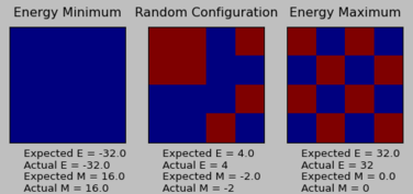
For each configuration, the expected energy and magnetisation values correspond exactly to the actual energy and magnetisation values. This confirms the accuracy of the energy() and magnetisation() functions in the IsingLattice script.
Section 3: Introduction to Monte Carlo simulation
Key ideas included in this section: The average energy and magnetisation functions are defined to evaluate a system of different configurations of spins. a) Large amount of time is required to compute a given system of all possible spin configurations. b) Importance sampling is imposed to only average states that can be generated with a certain probability distribution. c)The sampling is based on Metropolis Monte Carlo method, which only produce states with probability distribution equal to the Boltzmann factor; therefore, only statistically probable states are averaged.
TASK: How many configurations are available to a system with 100 spins? To evaluate these expressions, we have to calculate the energy and magnetisation for each of these configurations, then perform the sum. Let's be very, very generous, and say that we can analyse 1 x 10^9 configurations per second with our computer. How long will it take to evaluate a single value of <M>T ?
By observation, each cell can have 50:50 chances of either spin +1 or spin -1, there are 2 possible configurations per cell. In a lattice with 100 cells, the total number of possible configurations is 2100. Assuming that 109 configurations can be computed per second, then the time required for a lattice with 100 cells is 1.268 x 10²¹ seconds, which translates into 4.021 x 10¹² decades (4.0208 x 10¹³ years) to evaluate a single value of <M>T. This leads to the need to impose importance sampling in order to reduce the number of non-priority configurations for averaging.
TASK: Implement a single cycle of the above algorithm in the montecarlocycle(T) function. This function should return the energy of your lattice and the magnetisation at the end of the cycle. You may assume that the energy returned by your energy() function is in units of kB . Complete the statistics() function. This should return the following quantities whenver it is called: <E>, <E2>, <M>, <M2>, and the number of Monte Carlo steps that have elapsed.
The full documentation of source code can be found below:
import numpy as np
import math
class IsingLattice:

    E = 0.0
    E2 = 0.0
    M = 0.0
    M2 = 0.0

    n_cycles = 0

    def __init__(self, n_rows, n_cols):
        self.n_rows = n_rows
        self.n_cols = n_cols
        self.lattice = np.random.choice([-1,1], size=(n_rows, n_cols))

    def energy(self):
        "Return the total energy of the current lattice configuration."
        N = self.n_rows*self.n_cols
        spin_value = []
        for i in range (self.n_rows):
            for j in range (self.n_cols):
                #interactions (left)
                if j > 0:
                    spin_value.append(self.lattice[i,j]*self.lattice[i,j-1])
                else:
                    spin_value.append(self.lattice[i,j]*self.lattice[i,-1])
                #interactions (right)
                if j < self.n_cols-1:
                    spin_value.append(self.lattice[i,j]*self.lattice[i,j+1])
                else:
                    spin_value.append(self.lattice[i,j]*self.lattice[i,0])
                #interactions (top)
                if i > 0:
                    spin_value.append(self.lattice[i,j]*self.lattice[i-1,j])
                else:
                    spin_value.append(self.lattice[i,j]*self.lattice[-1,j])
                #interactions (bottom)
                if i < self.n_rows-1:
                    spin_value.append(self.lattice[i,j]*self.lattice[i+1,j])
                else:
                    spin_value.append(self.lattice[i,j]*self.lattice[0,j])

        total_energy = -0.5*(1.0)*sum(spin_value)
        return total_energy

    def magnetisation(self):
        "Return the total magnetisation of the current lattice configuration."
        magnetisation = []
        for i in range (self.n_rows):
            for j in range (self.n_cols):
                magnetisation.append(self.lattice[i,j])
        total_magnetisation = sum(magnetisation)
        return total_magnetisation

    def montecarlostep(self, T):
        # complete this function so that it performs a single Monte Carlo step
        #The original lattice corresponds to a0, the first configuration of spins with energy, E0. The self.energy function
        #will calculate the latest lattice generated so far, ie. the original_lattice.
        E0 = self.energy()
        M0 = self.magnetisation()
        #Generating the new lattice with one spin flipped. The random_i and random_j define the coordinates where the spin should be flipped
        #in the original lattice. Therefore the new_lattice specifies the coordinates with the reversed spin (ie. multiplication of -1).
        random_i = np.random.choice(range(0, self.n_rows))
        random_j = np.random.choice(range(0, self.n_cols))
        self.lattice[random_i, random_j] = self.lattice [random_i,random_j]*-1
        E1 = self.energy()
        M1 = self.magnetisation()
        #Finding the energy difference. random_number generates a value in range of 0 to 1.
        E_diff = E1 - E0
        random_number = np.random.random()
        # the self.n_cycles is placed here, because irrespective of the successful E1 values, each cycle is counted when
        # a spin of the original lattice is flipped.
        self.n_cycles = self.n_cycles + 1
        #The below function specifies the first condition where the energy difference is less than zero (ie. relaxation).
        #Relaxation processes are favoured and therefore thermodynamically allowed at all times. Taking the E1 value,
        #the running sums are updated and that the E2, M2 values are calculated.
        if E_diff < 0:
            self.E = self.E + E1
            self.M = self.M + M1
            E2 = E1*E1
            self.E2 = self.E2 + E2
            M2 = M1*M1
            self.M2 = self.M2 + M2
            return E1, M1
        else:
            Probability = math.exp(-E_diff/T)
            if Probability >= random_number:
                self.E = self.E + E1
                self.M = self.M + M1
                E2 = E1*E1
                self.E2 = self.E2 + E2
                M2 = M1*M1
                self.M2 = self.M2 + M2
                return E1, M1
            else:
                 self.lattice[random_i, random_j] = self.lattice [random_i, random_j]*-1
                # When E1 is rejected, the original energy E0 is added to the running sum instead.
                    self.E = self.E + E0
                    self.M = self.M + M0
                    E2 = E0*E0
                    self.E2 = self.E2 + E2
                    M2 = M0*M0
                    self.M2 = self.M2 + M2
                return E0, M0

        # the outputs at this step return successful E1 and M1 values, along with the running sums of E, E2, M and M2.
    def statistics(self):
        # complete this function so that it calculates the correct values for the averages of E, E*E (E2), M, M*M (M2), and returns them
        # the functions below calculate the final averages of E, E2, M and M2 based on the last running sum for each variable.
        Avg_E = self.E/self.n_cycles
        Avg_M = self.M/self.n_cycles
        Avg_E2 = self.E2/self.n_cycles
        Avg_M2 = self.M2/self.n_cycles
        return Avg_E, Avg_M, Avg_E2, Avg_M2, self.n_cycles
The purpose of the montecarlocycle function is to impose importance sampling to choose only the system microstates with the highest statistical probabilities, which are then used to compute <E>T ahd <M>T.
In summary, the code is based on statistical probability that a system microstate can exist in the given temperature. The original lattice is randomly generated using the energy() and magnetisation() defined above. This results in the initial energy and magnetisation values, E0 and M0. A subsequent lattice is generated by flipping one of the spins in the lattice via defining a random coordinate (i,j).
ΔE corresponds to the energy requirement to flip one of the spins in the lattice. Using this energy difference, the three conditions for the Monte-Carlo step can be defined:
(1) If ΔE < 0, the process of flipping a spin is energetically favourable, which corresponds to a high statistical probability that the particular microstate can exist.
(2) If ΔE > 0 and that the corresponding Boltzmann factor is greater than a random number in the interval [0,1), the transition is accepted due to fulfilling the probability requirement.
(3) If ΔE > 0 and that the corresponding Boltzmann factor is less than a random number in the interval [0,1), the transition is not energetically favourable and fail the importance sampling.
The statistics() function calculates the average of energy value, energy value squared, magnetisation value and magnetisation value squared. As the code progresses with each simulation, the transition that passes the importance sampling contributes to the running sums of energy and magnetisation values (if a transition is eliminated in the sampling, the original 'unflipped' lattice's energy and magnetisation values are added to the running sums instead). Each running sum is divided by the total number of Monte Carlo steps performed (ie. n_cycles).
TASK: If T < TC , do you expect a spontaneous magnetisation (ie. do you expect <math>\left\langle M\right\rangle \neq 0</math>)? When the state of the simulation appears to stop changing (when you have reached an equilibrium state), use the controls to export the output to PNG and attach this to your report. You should also include the output from your statistics() function.
TC is the Curie temperature, which corresponds a phase transition from ferromagnetism to paramagnetism. In paramagnetic materials, the magnetic dipoles are randomly oriented and therefore results in no net magnetisation. Therefore, for temperatures below the Curie temperature, net spontaneous magnetisation can be expected.
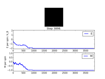
The output shown above corresponds to when equilibrium state is reached for a 8x8 lattice. Below the critical Curie temperature, a spontaneous magnetisation is expected from the lattice. As shown in previous sections, the ground states' energy is described by E = -DNJ. For a 8x8 2D lattice, the energy is equal to -2J.
NJ: per-spin Furthermore, the ground states are only achieved in lattice microstates where all spins are parallel. This corresponds to either +1 or -1 per spin in the lattice. The output from the statistics() function are:
E = -2.0
E*E = 4.0
M = 1.0
M*M = 1.0
The averaged values computed above are precise integral values given that large number of Monte Carlo Cycle computed, resulting in more homogeneous values.
Section 4: Accelerating the Code
Key ideas included in this section: The Monte Carlo step can be accelerated further using the numpy functions instead of using loop functions.
TASK: Use the script ILtimetrial.py to record how long your current version of IsingLattice.py takes to perform 2000 Monte Carlo steps.
| Recorded Time For Simulations (seconds) | |||
|---|---|---|---|
| 1st attempt | 5.8048498 | 6th attempt | 5.8435528 |
| 2nd attempt | 5.7740517 | 7th attempt | 5.8689594 |
| 3rd attempt | 5.8278122 | 8th attempt | 5.8642341 |
| 4th attempt | 5.8264647 | 9th attempt | 5.8434085 |
| 5th attempt | 5.8397669 | 10th attempt | 5.826643 |
| AVERAGE | 5.832274 | ||
| STD ERROR | 0.008222 | ||
TASK: Look at the documentation for the NumPy sum function. You should be able to modify your magnetisation() function so that it uses this to evaluate M. The energy is a little trickier. Familiarise yourself with the NumPy roll and multiply functions, and use these to replace your energy double loop (you will need to call roll and multiply twice!)
The revised energy() and magnetisation() functions are shown below:
<code>import numpy as np
import math
class IsingLattice:

    E = 0.0
    E2 = 0.0
    M = 0.0
    M2 = 0.0

    n_cycles = 0

    def __init__(self, n_rows, n_cols):
        self.n_rows = n_rows
        self.n_cols = n_cols
        self.lattice = np.random.choice([-1,1], size=(n_rows, n_cols))
        #the commands above generates a random lattice of size, n_rows x n_cols. Furthermore, the spin configuration is such that it is either
        # -1 or +1 in either cell.
    def energy(self):
        "Return the total energy of the current lattice configuration."
        sisj_horizontal = np.roll(self.lattice,1,axis=1)
        sisj_vertical = np.roll(self.lattice,1, axis=0)
        sisj_horizontal_energy = np.sum(np.multiply(sisj_horizontal,self.lattice))
        sisj_vertical_energy = np.sum(np.multiply(sisj_vertical,self.lattice))
       # the optimisation is performed using the numpy functions. The first command allows the end of the horizontal (row) array to be moved to
       # the front, which accounts for interactions between cells on the left edge with the right edge (ie. the next lattice). The same is applied
       # for the top row of the lattice, as the second command allows the top row of the lattice to interact with the adjacent lattice.
        E = -(sisj_horizontal_energy+sisj_vertical_energy)
       # the final energy function excludes 0.5 (originally included to account for double-counting) as only two rolled lattices interact with the original
       # lattice.
        return E

    def magnetisation(self):
        "Return the total magnetisation of the current lattice configuration."
        total_magnetisation = np.sum(self.lattice)
        # total magnetisation equals the sum of all the spin values ie. self.lattice
        return total_magnetisation
NJ: These comments are better Magnetisation() function is modified using np.sum , which eliminates the need for the inclusion of a double-loop to include all lattice cells. Energy() function evaluates interactions for cells adjacent to each other in a row, as well as interactions for cells adjacent to each other in a column. The np.roll function accounts for interactions for cells on the edges of the lattices with neighbouring lattices without additional loops. As a result of only accounting for two types of interactions in the accelerated code, the final energy equation does not account for the 0.5 factor.
TASK: Use the script ILtimetrial.py to record how long your new version of IsingLattice.py takes to perform 2000 Monte Carlo steps. This will vary, depending on what else the computer happens to be doing, so perform repeats and report the error in your average!
| Recorded Time for Accelerated Simulations (seconds) | |||
|---|---|---|---|
| 1st attempt | 0.140155383 | 6th attempt | 0.1363520515 |
| 2nd attempt | 0.142561794 | 7th attempt | 0.1361519211 |
| 3rd attempt | 0.140372904 | 8th attempt | 0.1358713966 |
| 4th attempt | 0.144783754 | 9th attempt | 0.1373073746 |
| 5th attempt | 0.134409191 | 10th attempt | 0.1362491398 |
| AVERAGE | 0.138421433 | ||
| STD ERROR | 0.00104 | ||
Section 5: The Effect of Temperature
Key ideas included in this section: At this point, the accelerated Monte Carlo step functions are defined after incorporating the numpy functions to highlight spins interactions. a) For a lattice system, each Monte Carlo step results in a different spin configuration for the lattice. b)Continuous increase in temperature allows the system to overcome energetic barrier to the most stable states. c) Subsequent Monte Carlo steps after this results in the same ground state, which contributes most to the average energetic and magnetisation values (the process of viewing the shift from a random to equilibrium configuration is done on ILfinalframe.py).
TASK: The script ILfinalframe.py runs for a given number of cycles at a given temperature, then plots a depiction of the final lattice state as well as graphs of the energy and magnetisation as a function of cycle number. This is much quicker than animating every frame! Experiment with different temperature and lattice sizes. How many cycles are typically needed for the system to go from its random starting position to the equilibrium state? Modify your statistics() and montecarlostep() functions so that the first N cycles of the simulation are ignored when calculating the averages. You should state in your report what period you chose to ignore, and include graphs from ILfinalframe.py to illustrate your motivation in choosing this figure.
NJ: Why did you take screenshots, rather than using the PNG exporter built into the plot window?
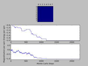
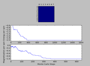
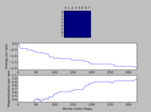
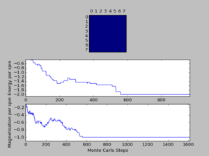
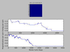
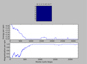
A total of six simulations on ILanim.py are ran to determine the minimum number of cycles required to reach the equilibrium final lattice state. All simulations are ran using 8x8 lattice with temperature = 1.0. The cutoff for n cycles is determined to be 1,600 as it is the largest number of cycles required to reach the equilibrium state, performed on all simulations shown above.The importance of the cutoff_cycles is due to its influence on determining the homogeneity of states with average energy and magnetisation properties. Removal of 1,600 Monte Carlo steps is expected to have minimal interference in the accuracy of the simulation, as it is a small percentage ( 1.06%) of the steps specified in ILfinalframe.py. There are associated anomalies with running the ILfinalframe.py which illustrates specific regions of opposite spins, corresponding to the lattice reaching a meta-stable state (an intermediary position along the reaction coordinate).
NJ: Why didn't you investigate different lattice sizes and temperatures?
The final statistics() is shown below:
<code>    def statistics(self):
        # complete this function so that it calculates the correct values for the averages of E, E*E (E2), M, M*M (M2), and returns them
        # the functions below calculate the final averages of E, E2, M and M2 based on the last running sum for each variable.
        if self.n_cycles > self.cutoff_n_cycles:
            Avg_E = self.E/(self.n_cycles - self.cutoff_n_cycles)
            Avg_M = self.M/(self.n_cycles - self.cutoff_n_cycles)
            Avg_E2 = self.E2/(self.n_cycles - self.cutoff_n_cycles)
            Avg_M2 = self.M2/(self.n_cycles - self.cutoff_n_cycles)
            return Avg_E, Avg_E2, Avg_M, Avg_M2, (self.n_cycles - self.cutoff_n_cycles)
        else:
        # for n_cycles within the cutoff_n_cycles range, there are no contributions to the running sums for E, E2, M and M2.
            print ('Within cutoff n cycles')
            return 0,0,0,0, self.n_cycles
The cutoff_n_cycles shown above is defined in earlier commands and it is also incorporated into the final montecarlo step shown below:
<code>def montecarlostep(self, T):
        # complete this function so that it performs a single Monte Carlo step
        #The original lattice corresponds to a0, the first configuration of spins with energy, E0. The self.energy function
        #will calculate the latest lattice generated so far, ie. the original_lattice.
        E0 = self.energy()
        M0 = self.magnetisation()
        #Generating the new lattice with one spin flipped. The random_i and random_j define the coordinates where the spin should be flipped
        #in the original lattice. Therefore the new_lattice specifies the coordinates with the reversed spin (ie. multiplication of -1).
        random_i = np.random.choice(range(0, self.n_rows))
        random_j = np.random.choice(range(0, self.n_cols))
        self.lattice[random_i, random_j] = self.lattice [random_i,random_j]*-1
        # the functions specified which cell will contain a flipped spin via coordinates. A new lattice results from flipping that spin.
        E1 = self.energy()
        M1 = self.magnetisation()
        #Finding the energy difference. random_number generates a value in range of 0 to 1.
        E_diff = E1 - E0
        random_number = np.random.random()
        # the self.n_cycles is placed here, because irrespective of the successful E1 values, each cycle is counted when
        # a spin of the original lattice is flipped.
        self.n_cycles = self.n_cycles + 1
        # function above monitors the running sum of the n_cycles.
        # defined the cutoff for n_cycles (the non equilibrated states).
        self.cutoff_n_cycles = 1600
        if E_diff < 0:
            # if the self.n_cycles is larger than the cutoff for n_ccyles then the values generated
            # contributed to the running sum, which will be contributed to the averages.
            if self.n_cycles > self.cutoff_n_cycles:
                self.E = self.E + E1
                self.M = self.M + M1
                E2 = E1*E1
                self.E2 = self.E2 + E2
                M2 = M1*M1
                self.M2 = self.M2 + M2
            return E1, M1
        else:
            Probability = math.exp(-E_diff/T)
            if Probability >= random_number:
                if  self.n_cycles > self.cutoff_n_cycles:
                    self.E = self.E + E1
                    self.M = self.M + M1
                    E2 = E1*E1
                    self.E2 = self.E2 + E2
                    M2 = M1*M1
                    self.M2 = self.M2 + M2
                return E1, M1
            else:
                self.lattice[random_i, random_j] = self.lattice [random_i, random_j]*-1
                if  self.n_cycles > self.cutoff_n_cycles:
                # When E1 is rejected, the original energy E0 is added to the running sum instead.
                    self.E = self.E + E0
                    self.M = self.M + M0
                    E2 = E0*E0
                    self.E2 = self.E2 + E2
                    M2 = M0*M0
                    self.M2 = self.M2 + M2
                return E0, M0
TASK: Use ILtemperaturerange.py to plot the average energy and magnetisation for each temperature, with error bars, for an lattice. Use your initution and results from the script ILfinalframe.py to estimate how many cycles each simulation should be. The temperature range 0.25 to 5.0 is sufficient. Use as many temperature points as you feel necessary to illustrate the trend, but do not use a temperature spacing larger than 0.5. T NumPy function savetxt() stores your array of output data on disk — you will need it later. Save the file as 8x8.datso that you know which lattice size it came from.
The full documentation of the ILtemperaturerange.py code can be found below, along with the codes specifying the standard error bars. The error bars are calculated by accounting for the net number of Monte Carlo steps used for the averaging process (eliminating the 1,600 Monte Carlo steps that do not result in homogeneous configurations).
Based on the results from the last section, the number of cycles for each simulation should be large enough so that finding the average properties for larger lattice can be as accurate as for the smaller lattices (the number of steps correlate to the number of simulations we can perform for each lattice cell). Furthermore, simulations of the ILfinalframe.py illustrate that at least 6000 steps are required to reach equilibrium state for the largest lattice (32x32). NJ: What results? You only looked at 1 lattice size...
A full documentation of the ILtemperaturerange.py code can be found below:
from IsingLattice import *
from matplotlib import pylab as pl
import numpy as np

n_rows = 32
n_cols = 32
il = IsingLattice(n_rows, n_cols)
il.lattice = np.ones((n_rows, n_cols))
spins = n_rows*n_cols
runtime = 100000
times = range(runtime)
temps = np.arange(0.25, 5.0, 0.3)
energies = []
magnetisations = []
energysq = []
magnetisationsq = []
net_cycles = []
for t in temps:
    for i in times:
        if i % 100 == 0:
            print(t, i)
        energy, magnetisation = il.montecarlostep(t)
    aveE, aveE2, aveM, aveM2, n_cycles = il.statistics()
# n_cycles described above already accounts for the elimination of 1,600 cycles that do not result in average lattice properties described in
#IsingLattice.py statistics() function.
    energies.append(aveE)
    energysq.append(aveE2)
    magnetisations.append(aveM)
    magnetisationsq.append(aveM2)
    net_cycles.append(n_cycles)
    #reset the IL object for the next cycle
    il.E = 0.0
    il.E2 = 0.0
    il.M = 0.0
    il.M2 = 0.0
    il.n_cycles = 0
fig = pl.figure()
enerax = fig.add_subplot(2,1,1)
enerax.set_ylabel("Energy per spin")
enerax.set_xlabel("Temperature")
enerax.set_ylim([-2.1, 0])
magax = fig.add_subplot(2,1,2)
magax.set_ylabel("Magnetisation per spin")
magax.set_xlabel("Temperature")
magax.set_ylim([-1.1, 1.1])
enerax.plot(temps, np.array(energies)/spins)
magax.plot(temps, np.array(magnetisations)/spins)

energies_y = np.array(energies)/spins
magnetisation_y = np.array(magnetisations)/spins

#the commands below generate corresponding energies and magnetisations error bars using the relationship of <E2> and <E>^2 in standard deviation.
#only the Monte-Carlo steps that are not cut off in the entire cycles are considered for the error bars.
standard_error_energies = np.sqrt(np.array(energysq) - (np.array(energies)*np.array(energies)))/np.sqrt(np.array(n_cycles))
standard_error_magnetisation = np.sqrt(np.array(magnetisationsq) - (np.array(magnetisations)*np.array(magnetisations)))/np.sqrt(np.array(n_cycles))

enerax.errorbar(temps,np.array(energies)/spins,yerr=standard_error_energies, linestyle="None")
magax.errorbar(temps,np.array(magnetisations)/spins,yerr=standard_error_magnetisation, linestyle="None")

pl.show()
final_data = np.column_stack((temps, energies, energysq, magnetisations, magnetisationsq))
np.savetxt("32x32.dat", final_data)
The 8x8 lattice's energetic and magnetic values are shown below, which are generated using 0.3 interval between each temperature point from range 0 to 5.0. Magnitudes of the error bars depend directly on the number of n_cycles stated on the code above (n_cycles accounted for the 1,600 Monte Carlo steps that are being cut off from the total number of steps). The number of steps chosen for this simulation is sufficiently large given that the fluctuations are being captured for both energetic and magnetic values, along with the phase transitions. For the purpose of accuracy, it is important to impose cut off cycles that are as small as possible, due to the need for larger lattices to have longer steps. As the lattice size increases, the errors associated becomes larger for a given number of n_cycles. This is due to the fact that less simulations are performed per cell.

Section 6: Scaling the System Size
Key ideas included in this section: The previous section generates individual data file for each lattice size. Energy and magnetisation values in the data file can therefore be used to show unique fluctuations for every lattice size. From this, there is a need to determine the minimum lattice size required to capture energy and magnetisation fluctuations from temp = 0 to temp 5.0. a) Demonstrated that the fluctuations of the 8x8 lattice are similar to the larger sized lattices b) temperature peaks on the magnetisation curve illustrate phase transitions such that the entropic and energetic driving forces are equal at this point.
TASK: Repeat the final task of the previous section for the following lattice sizes: 2x2, 4x4, 8x8, 16x16, 32x32. Make sure that you name each datafile that your produce after the corresponding lattice size! Write a Python script to make a plot showing the energyper spin versus temperature for each of your lattice sizes. Hint: the NumPy loadtxt function is the reverse of the savetxt function, and can be used to read your previously saved files into the script. Repeat this for the magnetisation. As before, use the plot controls to save your a PNG image of your plot and attach this to the report. How big a lattice do you think is big enough to capture the long range fluctuations?
The full documentation of temperature versus energy and magnetisation values can be found here:
from IsingLattice import *
import numpy as np
from matplotlib import pylab as pl
size = [2,4,8,16,32]
#plot_energy_curve extracts the required information for plotting E. Every energy value is converted to a per spin basis.
def plot_energy_curve (i):
	data = np.loadtxt(str(i) + 'x' + str(i) + ".dat")
	temp = data [:,0]
	energy = data [:,1]
	energy_per_spin = energy/(i*i)
	return temp, energy_per_spin
# defined the function required for plotting by looping every element in the size array to find the corresponding file.
for i in size:
	temp, energy_per_spin = plot_energy_curve(i)

	pl.plot(temp,energy_per_spin, label = str(i) + 'x' + str(i))
	pl.legend(loc='upper left')

	pl.ylabel("Energy per spin")
	pl.xlabel("Temperature")
	pl.title('Energy_per_spin')
pl.show()

def plot_magnetisation_curve (k):
	data = np.loadtxt(str(k) + 'x' + str(k) + ".dat")
	temp = data [:,0]
	magnetisation = data [:,3]
	magnetisation_per_spin = magnetisation/(k*k)

	return temp, magnetisation_per_spin

for k in size:
	temp, magnetisation_per_spin = plot_magnetisation_curve(k)

	pl.plot(temp, magnetisation_per_spin,label = str(k) + 'x' + str(k))
	pl.legend(loc='upper left')

	pl.ylabel("magnetisation per spin")
	pl.xlabel("Temperature")
	pl.title('magnetisation_per_spin')
pl.show()

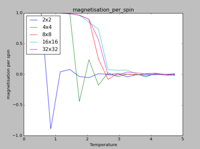
The Energy_per_spin plot illustrates that decreasing temperature leads to a value of -2, which corresponds to the ground state energy (total) calculated in previous section, where E = -4NJ for a two-dimensional lattice.
NJ: E=-2NJ
Given that flipping one spin in larger lattices from ground states incurred less energetic change, the 2x2 lattice requires higher temperature to reach the same energetic value as other lattices.
NJ: The energy change when flipping one spin will be the same no matter what the lattice size is. What you're observing is the that "phase transition" in the very small lattice (2x2) takes places over a much larger temperature range than in the larger lattices.
Furthermore, the magnetisation_per_spin curve also suggests that the temperature at which phase transitions occur changes according to lattice size. This temperature point indicated as the peaks of each magnetisation curve, where it signals a phase transition to paramagnetism. Based on the magnetisation_per_spin graph, it is evident that lattices of size 8x8 are large enough to capture long-range fluctuations as the values plateau quicker for lattices of greater sizes. Furthermore, the 8x8 lattice tends to similar fluctuations for the larger sized lattices.
Section 7: Determining the Heat Capacity
Key ideas included in this section: The heat capacity can be shown to be related to the variance of the average energy, <E>. Using corresponding data file from previous sections, the relationship between lattice sizes and heat capacities can be derived. Furthermore, like any other phase transitions, there should points of discontinuity or divergence. The results from this section illustrate that there is a trend of divergence for larger lattice size, and as a result, it can be concluded that the transition to net magnetisation is second-order phase transition.
TASK: Find the relationship between heat capacity and Var[E]
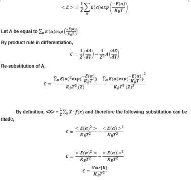
NJ: Be careful with your notation, some of those powers look like they're only applied to one term.
TASK: Write a Python script to make a plot showing the heat capacity versus temperature for each of your lattice sizes from the previous section. You may need to do some research to recall the connection between the variance of a variable, Var [E] , the mean of its square , <E2> and its squared mean <E> . You may find that the data around the peak is very noisy — this is normal, and is a result of being in the critical region. As before, use the plot controls to save your a PNG image of your plot and attach this to the report.
The variance is expressed as: Var[E] = <E2> - <E>2 . The full documentation of the code can be found below:
from IsingLattice import *
import numpy as np
from matplotlib import pylab as pl
#The size array will be used for a loop function to call out each file.
size = [2,4,8,16,32]
#Heat_capacity curve function extracts the required energetic values, which are used to calculate the variance values.
def heat_capacity (i):
	data = np.loadtxt(str(i) + 'x' + str(i) + ".dat")
	temp = data [:,0]
	E = data [:,1]
	E2 = data [:,2]
	M = data [:,3]
	M2 = data [:,4]

	variance_energy = np.array(E2)-(np.array(E)*np.array(E))
	C = variance_energy/(2**temp)

	return temp,C

for i in size:
	temp, C = heat_capacity(i)
# for every element of the size array, the corresponding file will be opened, extracted then plotted.
	pl.plot(temp,C, label = str(i) + 'x' + str(i) )
	pl.legend(loc = 'upper right')

	pl.ylabel("Heat Capacity")
	pl.xlabel("Temperature")
	pl.title('Heat Capacities of Lattice Sizes')
#no indentation in the following behind allows all graphs to be in the same figure.
pl.show()
The figure below illustrates the differences in heat capacities of various lattice sizes. As the lattice size increases, it becomes evident that the heat capacity becomes greater as there are greater number of cells to absorb thermal energy required for the phase transition, as heat capacity is an extensive property.
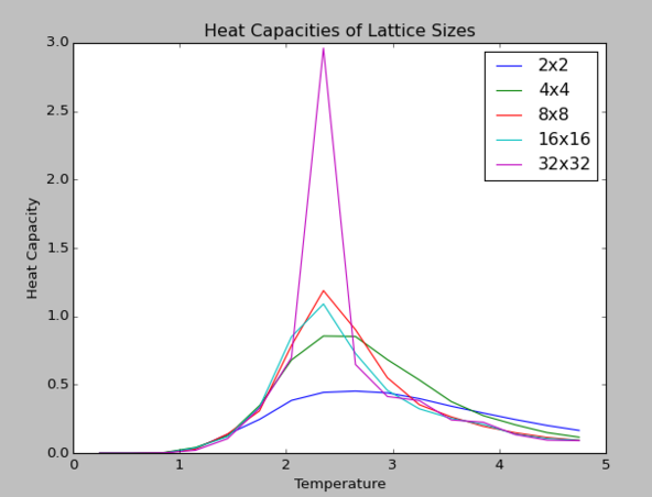
As shown above, there is a rapid logarithmic divergence in the heat capacity values as the lattice size increases.
Section 8: Locating the Curie Temperature
TASK: A C++ program has been used to run some much longer simulations than would be possible on the college computers in Python. You can view its source code here if you are interested. Each file contains six columns: (the final five quantities are per spin), and you can read them with the NumPy loadtxt function as before. For each lattice size, plot the C++ data against your data. For one lattice size, save a PNG of this comparison and add it to your report — add a legend to the graph to label which is which. To do this, you will need to pass the label="..." keyword to the plot function, then call the legend() function of the axis object (documentation here).
The comparison of 8x8 lattice's heat capacity between the Python data and the C++ data are shown below:
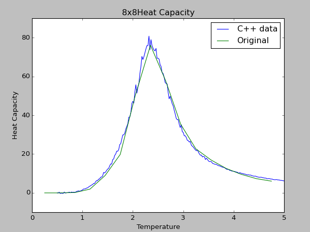
As shown, the 'Original' curve corresponds to the 8x8.dat Python file, which shows close approximation to the C++ data. To ensure that the two curves are of the same magnitude, the energetic and magnetic values from each Python and C++ sources are calculated on a per spin basis. Given that the C++ data are generated from longer simulations, the curve generated is more defined by comparison to the Python data source. The full documentation of the Heat Capacity curve can be found below (HeatcapacityplotC++.py):
from IsingLattice import *
import numpy as np
from matplotlib import pylab as pl

#The array 'size' is used later for flexible loop function to call out corresponding nxn files.
size = [2,4,8,16,32]
#The function below defines the commands to read the C++ files to extract temperature and
#Heat capacity data.
def heat_capacity_C (i):
	# All C++ files have been migrated outside of the C++ data file and renamed as nxn v2
	data = np.loadtxt(str(i) + 'x' + str(i) + " v2" + ".dat")
	temp_new = data [:,0]
	E = data [:,1]
	E2 = data [:,2]
	C = data[:,5]

	C_new = np.array(C)

	return temp_new,C_new
#The function below defines the commands to read the Python files to extract temperature and  data.
def heat_capacity (i):
	data = np.loadtxt(str(i) + 'x' + str(i) + ".dat")
	temp = data [:,0]
	E = data [:,1]
	E2 = data [:,2]
	M = data [:,3]
	M2 = data [:,4]

#Unlike in C++ file, the variance for energy must be calculated separately using the following commands.
	variance_energy = np.array(E2)-(np.array(E)*np.array(E))
	C = variance_energy/(2**temp*i*i)
# the values of C must be converted to be in a per spin basis, so that it is in the same magnitude as the C++ files.
	return temp,C

for i in size:
#The loop enables each n*n file to be read in order. For an element in 'size', the corresponding
#data will be extracted using the heat_capacity_C and heat_capacity functions.
	temp_new, C_new = heat_capacity_C(i)
	temp, C = heat_capacity(i)
#The plot functions are defined below.
	line1 = pl.plot(temp_new, C_new, label = 'C++ data')
	line2 = pl.plot(temp,C, label = 'Original')

	pl.legend(loc='upper right')


	pl.ylabel("Heat Capacity")
	pl.xlabel("Temperature")
	pl.title(str(i) +  'x' + str(i) + 'Heat Capacity')
	pl.show()
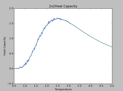
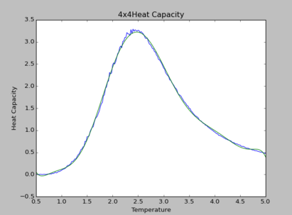
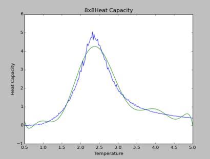
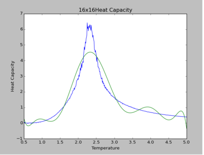
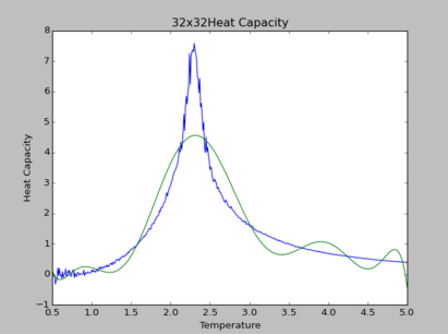
TASK: write a script to read the data from a particular file, and plot C vs T, as well as a fitted polynomial. Try changing the degree of the polynomial to improve the fit — in general, it might be difficult to get a good fit! Attach a PNG of an example fit to your report.
To produce a fitted polynomial to any of the heat capacity curve generated by the C++ data source, the following code is used:
from IsingLattice import *
import numpy as np
from matplotlib import pylab as pl

size = [2,4,8,16,32]

# Step 1: Extract the data from any given C++ file. Every data file's values are on a per spin basis.
def data_read(i):
	data = np.loadtxt(str(i) + 'x' + str(i) + ' v2' + ".dat")
	temp = data [:,0]
	C = data[:,5]
	C_allspins = C*(i*i)

	return temp, C_allspins

for i in size:
	temp, C_allspins = data_read(i)

	T_min = np.min(temp)
	T_max = np.max(temp)
	Temp_range = np.linspace(T_min, T_max, 1000)
	Temp_plot = np.array(Temp_range)

	fit = np.polyfit(temp, C_allspins, 9)
	fitted_C_values = np.polyval(fit, Temp_plot)

	line1 = pl.plot(temp, C_allspins)
	pl.plot(Temp_plot, fitted_C_values)

	pl.ylabel("Heat Capacity")
	pl.xlabel("Temperature")
	pl.title(str(i) + 'x' + str(i) + 'Heat Capacity')
	pl.show()
The polynomial of degree 9 produces the best fit for all simulations. By observation, at higher lattice sizes, the polynomial fittings become due to the curvature of polynomial fittings at extremes of the temperature range.
NJ: I don't understand what this sentence means.
TASK: Modify your script from the previous section. You should still plot the whole temperature range, but fit the polynomial only to the peak of the heat capacity! You should find it easier to get a good fit when restricted to this region.
The full documentation of the modified code for polynomial fitting can be found below:
NJ: Include some examples of these new fits.
<code>from IsingLattice import *
import numpy as np
from matplotlib import pylab as pl

size = [2,4,8,16,32]

# Step 1: Extract the data from any given C++ file
def data_read(i):
	data = np.loadtxt(str(i) + 'x' + str(i) + ' v2' + ".dat")
	temp = data [:,0]
	C = data[:,5]
	C_allspins = C*(4)

	return temp, C_allspins

for i in size:
	temp, C_allspins = data_read(i)

	T_min = 2.0
	T_max = 2.8
	selection = np.logical_and(temp > T_min, temp < T_max)

	Temp_range = np.linspace(T_min, T_max, 1000)
	Temp_plot = np.array(Temp_range)
	peak_T_values = temp[selection]
	peak_C_values = C_allspins[selection]
	fit = np.polyfit(peak_T_values, peak_C_values, 9)

	fitted_C_values = np.polyval(fit,peak_T_values)

	line1 = pl.plot(temp, C_allspins)


	pl.plot(peak_T_values, fitted_C_values)
	pl.ylabel("Heat Capacity")
	pl.xlabel("Temperature")
	pl.title(str(i) + 'x' + str(i) + 'Heat Capacity')
	pl.show()
TASK: find the temperature at which the maximum in C occurs for each datafile that you were given. Make a text file containing two colums: the lattice side length (2,4,8, etc.), and the temperature at which C is a maximum. This is your estimate of for that side length. Make a plot that uses the scaling relation given above to determine . By doing a little research online, you should be able to find the theoretical exact Curie temperature for the infinite 2D Ising lattice. How does your value compare to this? Are you surprised by how good/bad the agreement is? Attach a PNG of this final graph to your report, and discuss briefly what you think the major sources of error are in your estimate.
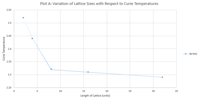
| Length of Lattice | Temperature Corresponding to
Maximum Heat Capacity (in units of J) |
|---|---|
| 2 | 2.52 |
| 4 | 2.44 |
| 8 | 2.32 |
| 16 | 2.31 |
| 32 | 2.29 |
The relationship between the Curie temperature and the lattice size is determined by the following equation:
NJ: You should instead have made a plot of T vs 1/L. This graph is linear, and the value that you want is the intercept. How did you do your extrapolation? Where does the error come from? You should have made this plot using Python, not Excel.
Using the simulations above, the empirical results yield the trend below. Given 1/L dependence in the equation for finding Curie temperature for infinite lattice size, it is expected that the Curie temperature tends to a singular temperature value. In the analysis below, extrapolation indicates that the experimental value is 2.28. This is in close agreement with the literature value[1], which states that an infinite lattice has a critical point at Curie Temperature, TC = 2.269.
NJ: Your reference doesn't offer any proof that this value is correct, it simply quotes it. You should find a literature value instead.
The resultant experimental error is 0.04%, owing to a number of factors.
NJ: Where does this come from? Is your result within error or not?
A foremost contribution to the error is from the cutoff number of cycles defined earlier in plotting energy and magnetisation values with respect to temperature for each lattice size (codes are specified in the ILtemperaturerange.py file).
NJ: If this error was a big problem, your graphs of energy and magnetisation per spin would also be affected - do you think they are wrong?
Inclusion of fewer Monte Carlo steps in the process of finding the average properties, result in averaging states that do not possess average energetic and magnetic values, which can influence the accuracy of subsequent simulations.
To confirm this possible observation, further ILanim.py simulations are ran for 32x32 lattices, which indicated that 5000 Monte Carlo steps are required before reaching a configuration corresponding to equilibrium.
A second contribution to the error results from defining the degree of polynomial fitting, as the polynomial fittings are subsequently used to determine the maximum heat capacities and corresponding temperatures. Finally, the extrapolation to determine the Curie temperature for infinite lattice remains an estimation based on 32x32 sized lattice. For the purpose of future accuracy, it is recommendable that larger lattice sizes are inputted into the simulation, so that there are more data points for the trend line.
- ↑ K.J Beers, Numerical Methods for Chemical Engineering: Applications in MATLAB, Cambridge University Press, 2007, pg. 357,

