Talk:Mod:CMPAlexCard
Programming for Liquid Simulation
The Ising Model & Phase Transition
Task 1
Finding the general solution for the lowest enthalpic energy of a magnetic lattice by inspection is trivial. The lowest energy solution corresponds to a perfect ferromagnetic lattice. That is, all the spins of each lattice unit is aligned in the same direction, either all up or all down. This is clear because arranging the system in such a way gives the summation term the largest possible positive value. Thus, when calculating the sum of along a certain direction in the lattice, the result will always be 2N, where N is the number of lattice units upon which the sum is evaluated. This is because every value of takes the value of 1 (or -1). The summation needs to be performed, however, in each orthogonal direction for every dimension of the lattice. That is, only once for a 1D lattice, but 3 times for a 3D lattice (in the x, y & z direction). Thus, the number of dimensions, D, needs to be multiplied by 2N to give the total enthalpic contribution. Put another way, a 1D crystal has only 2 neighbouring interactions, a 2D has 4, and a 3D posseses 6, thus it is a simple matter of multiplying the number of neighbouring interactions by the number of particles (and then dividing by 2 to eliminate doubly counted interactions) to obatain the same result. Entering this result into the Ising formula gives .
Calculating the number of possible micro-states in this configuration is also straight forward. Since there are N distinguishable particles in a solid lattice, all with the same spin state, only one micro-state is possible. However, the spins can either be all up or all down, giving a total multiplicity of two. Using the Boltzmann formula, , where W is the number of micro-states, the entropy can be easily calculated. The entropy using this formula, arising from purely magnetic contribution, is , or essentially zero. This is clearly its minimum possible value.
Task 2
The ground state energy of is . The energy of the lattice with one spin changed can be calculated by subtracting the stabilisation from 3 rows of 10 leading to a vertex, and adding back the stabilisation of three rows, conceptually where each row is oriented along the x. y & z axis with the spin-change unit at the vertex. That is, subtract where all spins are 1, and add where 1 in each sum contains a spin = -1. This gives: . Hence, the increase in energy is . A much simpler way to envisage this would be to consider the fact that 6J stabilisation energy is lost, and 6J destabilisation energy is gained in changing one spin in a 3D lattice. This is due to the fact that each unit has 6 neighbours in the simple 3D lattice.
Task 3

The magnetisation for the 1D and 2D lattices shown on the right are simply the sum of the individual spins, which sums to be the same in this case.
A lattice with 1000 units at absolulte zero would obviously not have any energy to overcome a spin-flip barrier, and would maximise its enthalpic energy by having all spins parallel, and thus .
NJ: or M=-1000
Calculating the Energy & Magnetisation of a 2D grid
A general computational solution is necessary for calculating the energy and magnetisation of an grid. The 2D grid is easily described by an array in python. The magnetisation is trivial, since all number in the array must simply be summed. This was done by first adding together the columns in each array, and then summing the remaining row.
Calculating the energy is more difficult to conceive, but has a neat solution. A while loop, with the condition that it is terminated when the final row has been reached, is set up. After each row has been looped over, a conditional if statement resets the value of the column counter to zero, and increases the row counter by one so that the next row may be looped over. At each point in the calculation, the multiple of all 4 neighbours of the item is calculated and added to variable "energy". The code was than implemented into the IsingLattice class, and tested using the ILcheck.py file with success.
The code and its results, in isolation from the class of IsingLattice, is shown as follows, where the is attributed to grid = Lattice(n_rows,m_cols) :
Task 4 & 5
| Magnetisation | Energy |
|---|---|
  def Mag(array):
    col_sum = sum(array)
    magnetisation = sum(col_sum)
    return magnetisation
|
def Energy(array):
    grid = array
    energy = 0
    rows = 4
    cols = 4
    c = 0
    r = 0

    while r < rows:
        energy += -0.5 * grid[r,c] * (grid[r,c-cols+1] + grid[r,c-1] + grid[r-rows+1,c] + grid[r-1,c])
        c += 1
        if c==cols:
    	    c,r = 0, r+1
    return energy
|
NJ: Good. Using a for loop is considered more "Pythonic" for a finite list. You should include some comments to explain the method, as well.
Task 6
The code was then checked with the ILcheck.py file, with the following results:
The formula derived by inspection earlier holds valid for the computationally calculated energy of the perfectly ordered system. That is, a value of . I also created a maximum energy lattice, to further validate the code that I had written. The result was also in agreement with that of the ILcheck.py file:
| Code & Result |
|---|
import numpy as np from numpy import * def Lattice_max(): lat = array ([(1,-1,1,-1),(-1,1,-1,1),(1,-1,1,-1),(-1,1,-1,1)]) return lat print Lattice_max() print 'Magnetisation = ' + str(Mag(grid)) print 'Total energy = ' + str(Energy(grid)) |
[[ 1 -1 1 -1] [-1 1 -1 1] [ 1 -1 1 -1] [-1 1 -1 1]] Magnetisation = 0 Total energy = 32.0 [Finished in 0.1s] |
Monte Carlo Simulation
Task 7: Average Energy and Magnetisation
The number of configuration for 100 different spins is , the value of which is 1267650600228229401496703205376. If we were able to calculate configurations per second, the time to complete all possible combinations would be 1267650600228229401496 seconds. Or, 40169423537538 years, much older than any computer or the universe. Though, on this laptop, the time actually taken to calculate the magnetisation for a 100 spin grid lattice is reported as 0m0.028s , meaning I can only perform the full set much slower than that still. Therefore, importance sampling is used to significantly reduce the problem.
Task 8: Importance Sampling
The Monte Carlo algorithm is employed in order to sample only the significant configurations of the many many possible. It does this by randomly creating a new configuration by making a single change to one item in the system, and accepting only those new configurations which either decrease the energy, or increase it with some realistic feasibility. That is, the system may contain enough thermal energy to populate some less energetically stable configurations, and these must be included. Those configurations, however, which represent a very large energy increase will be rejected all together. A single step of the algorithm is outlined below, assuming the energy Energy() and magnetisation Mag() functions are defined elsewhere:
| Monte Carlo cycle | Spin-change Alternative |
|---|---|
E0 = Energy(alpha0)
random_i = np.random.choice(range(1, len(alpha0) ))
random_j = np.random.choice(range(1, len(alpha0[0]) ))
alpha1 = deepcopy(alpha0)
alpha1[random_i][random_j] = -alpha1[random_i][random_j]
E1 = Energy(alpha1)
delE = E1 - E0
random_number = np.random.random()
new_config = []
if delE < 0:
    new_config = alpha1
    print '1. accept immediately'
else:
    if (2.71828182846**(-delE / T)) < random_number:
        new_config = alpha1
        print '2. accept energy increase'
    else:
        new_config = alpha0
        print '3. reject - return to initial'
alpha0 = new_config
E += Energy(new_config)
E2 += (Energy(new_config))**2
M += Mag(new_config)
M2 += (Mag(new_config))**2
n_cycles += 1
|
def random_spin_flip(array):

    alp0 = array
    single_list = np.arange( len(alp0)*len(alp0[0]) )
    rand_list = np.random.permutation(single_list)
    new = []
    for i in rand_list:
        if i != 0:
            i=1
            new.append(i)
        else:
            new.append(-1)

    new_spin_array = np.reshape((new),(len(alp0) , len(alp0[0])))
    return new_spin_array
|
The above code is in isolation from the class IsingLattice, so is slightly different in that it uses no self. notation, and employs deepcopy() in order to create a distinct value copy of alpha0, without which the code did not work. Additionally, an alternative method for randomly flipping one spin is shown above. This is slower, but seems relevant to include as I developed it first. It returns an array of 1s of the same dimension of self.lattice with a -1 placed at random, which can be used to np.multiply the original to flip one spin.
In the IsingLattice class, ultimately, no deepcopy() was necessary, and in order to return the flipped spin to its original state in the case that the new configuration was rejected, the random_j and random_i were recalled and used to re-flip the spin, thus returning to the initial configuration. This is a much simpler and computationally neat alternative, which is also favourable since it is quicker than deepcopy(). This is because it must make a replicated value copy, rather than simply recalling already defined values, random_j and random_i.
NJ: Good. deepcopy() was a nice idea, even though it turns out to be inefficient.
Task 9: Results of the Monte Carlo Algorithm
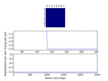
The check file ILanim.py was run for 2000 steps, with the following output:
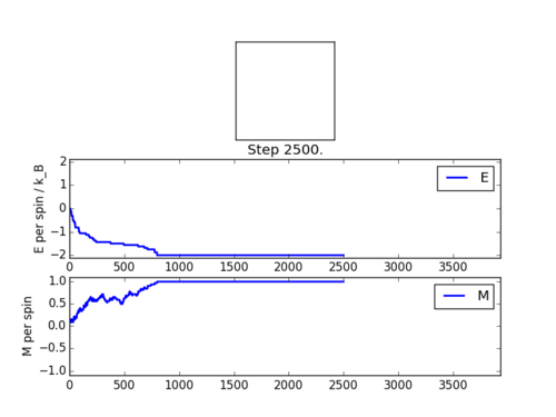
The statistics produced after these 2500 steps were as follows:
Averaged quantities:
('E = ', -1.8032726377952757)
('E*E = ', 3.3785602239173227)
('M = ', 0.8784448818897638)
('M*M = ', 0.8173420583169292)
In order to further calidate this, a Monte Carlo simulation for a 5 by 5 lattice was run with 1,000,000 steps via a while loop which is significantly faster in the absence of having to plot the graphics. The outline of the code, which takes number of cycles and temperature as arguments, is:
def Monte_carlo(T,cycles):
      while n_cycles < cycles:
          {Monte Carlo Algorithm}
      n_cycles += 1
      return mean energy per spin, mean magnetisation per spin
The results after 1,000,000 steps were more indicative of the convergence to the value of -2 for the mean energy per spin, which is clearly the case on the graphic on the right:
mean energy per spin = -1.99991104
mean mag per spin = -0.99995328
Both of the above Monte Carlo algorithms were run at 0.5 K. This temperature is very likely to be well below the curie temperature, so it would make sense that an overall magnetisation would predominate. The above results fit with this prediction. In general, at , the lattice will adopt a magnetisation, assuming it is in an equilibrium state, since there is not enough thermal energy to increase the entropy of the system.
A More Time-Efficient Algorithm
The current algorithm appears to work, though there is a large time penalty in calculating the energy. Not only because each individual element is looped through, but for each element 4 multiplications are calculated. This method inherently calculates each neighbouring spin interaction twice, which is clearly a misuse of computation. Another method is available, which calculates only the necessary number of spin interactions. That is, 2 per spin. Two separate modifications were made, with each significantly reducing the time taken to calculate the energy. The magnetisation was also sped up, on such a way that all the elements are summed at once, rather than summing the rows and columns separately.
Task 10, 11 & 12
In order to test the speed, multiple runs of the ILtimetrial.py file were run, with the results recorded in a file "time_trial" and later averaged. This was easily implemented 100 times using the linux terminal command:
for n in {1..100}; do python ILtimetrial.py >> time_trial; done
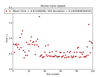
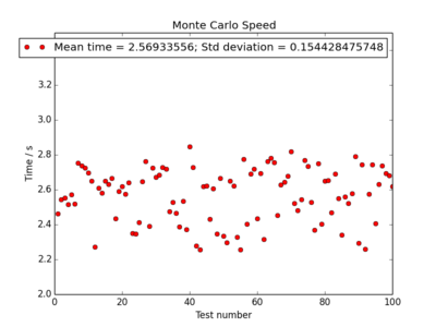
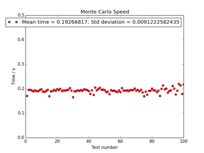
Each point on the plots correspond to 2000 Monte Carlo steps having been completed, as implemented in the ILtimetrial.py. The mean values for the time and their standard deviation's are given. The results, with the corresponding code for each energy calculation method, are shown below. The fastest method for calculating the energy makes use of the axis keyword which eliminates the need for the time-expensive for loop, and is over 20 times more efficient than the original code.
NJ: Very thorough, well done. Again, I would like to see a few comments within the code.
The Effect of Temperature
Task 13
It was demonstrated earlier that the mean energy after many multiple Monte Carlo steps only approaches the value to which it actually converges after about 1,000,000 steps. This number is quite costly in terms of time, so the code was altered to only start calculating the energy and magnetisation statistics after an arbitrary number of steps. In this case, 1000. The code is as follows:
This number was chosen because after 1000 steps the system had always undisputedly reached its equilibrium point for 0.5 K. It often reached this value at a lower value, often after only ~150 steps or less (as shown above), though to be certain, 1000 was used.
Task 14
The ILtemperaturerange.py file was then implemented to plot the average energy of an 8 by 8 grid over a range of temperatures, using the above correction to calculate the average energy. Some important alterations were made to this file, however. The bulk of these alteration were implemented to create variable error bars on the values for average energy and magnetisation. In this case, the error bars are simply the standard deviation, found from the set of values used to calculate the mean value. This was done using the numpy.std() function. At each point in the for loop for each temperature, the set of energy values (and equally, magnetisation) were appended to a list, from which the standard deviation was derived. At the end of the loop, the list of energies is re-defined as empty, ready for the next set of energies to be appended at the next temperature at which the lattice is evaluated.
I deliberately chose to use the standard deviation, , as a measure of error in the mean values, as opposed to the standard error. This is because the number of values used to calculate the mean energy is so large (50000) that the standard error, , would become vanishingly small with the square root of system size the denominator. Thus, it would convery little meaning when displayed on the graph.
The results are as follows. To create this plot, 20000 steps were performed for each value of temperature, for which intervals of 0.1 K were used in the range 0.5 to 5.0:
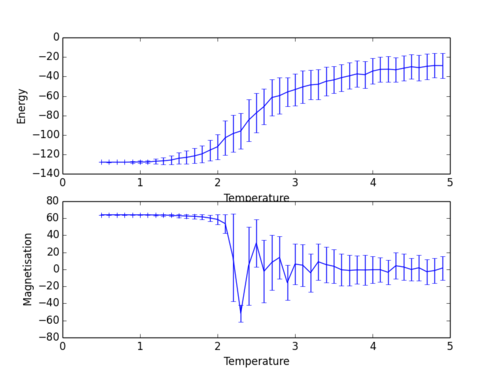
The size of the error bars reflect the variation about the system's equilibrium state for each given temperature. As expected, and as already seen above, the variation about the equilibrium state for low temperatures (i.e 0.5 K) is minimal. That is, the system does not have enough thermal energy to reach a state of higher entropy in favour of less enthalpic stability derived from the alignment of spins.
As the temperature increases, more variation is present as more configurations of higher disorder are accepted by the Monte Carlo algorithm. This greater value of standard deviation persists even as the systems appears to level out at T = 5 K, since there is still greater thermal energy to effect more variation in the system, even if an entropy / enthalpy balance has been struck. It is also apparent that the largest variation appears in the region where the average energy is changing.
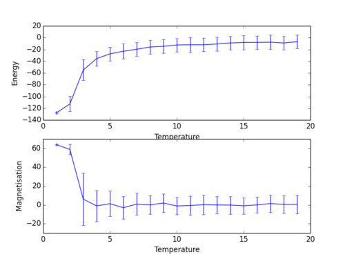
To illustrate further that a balance between enthalpic stabilisation of spin alignment and entropic favoured disorder has been struck, the test was tun again with fewer steps (10000) but from 1 to 20 K, with 1 K intervals.
Effect of System Size
Task 15
A range of system sizes were used to calculate their mean energies and magnetisation, over the same temperature range as before (0.5 K to 5.0 K). In this was the behaviour of the system at the onset of the phase transition can be contrasted. That is, at the point where entropic driving forces begin to interfere with enthalpic stability, large fluctuations can occur though only in system of a relatively larger size. Below, a range of 5 system sizes have their corresponding plots shown for both their average energy and magnetisation per spin.
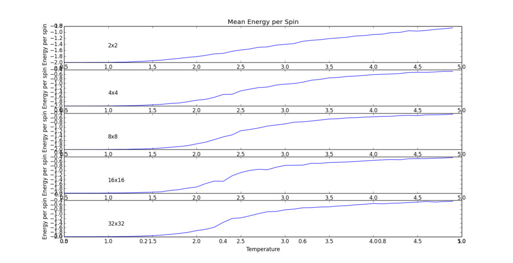
Script used : Lattice-var_temp_range.py
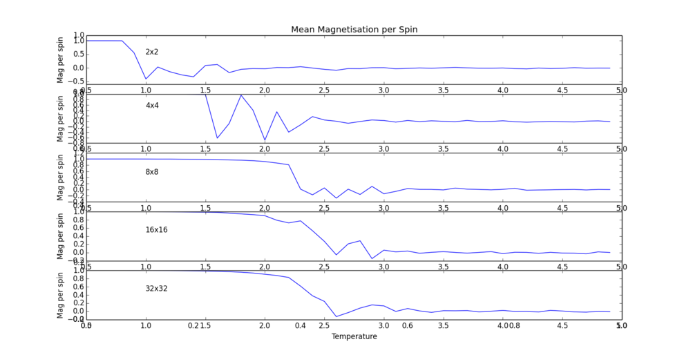
Script used : Lattice-var_temp_range.py
The phase transition in the system is most clearly seen in the magnetisation per spin. This clearly shows the transition from a value of 1 (all spins aligned in a very low-entropy system) to a value of zero (greater system entropy in favour of magnetic stability) as the temperature increases. However, there are differences in the temperature range over which the transition occurs. There is a fairly sharp change for the small 4 spin matrix at 0.8 K. Between the 16 and 64 spin matrix, the onset of the phase transition moves a significant gap, from 1.5 K to 2.25 K. byt the time the 32 by 32 (1024 spin) matrix has been reached, quite a broad transition is seen, within the range 1.5 to 2.5. To make this contrast even further, one more run was performed on a system with 10000 spins.
NJ: It's much easier to see the trend if these are all plotted on one graph. When doing this, it becomes clearer that an 8x8 lattice gives very similar results to a 16x16 or 32x32.
Determining the Heat Capacity
Task 16
The value of the heat capacity is quite easily determined, since it is related to the variance of the internal energy of a system. The variance is easily caclulated from the statistical relationship , where in our case the X represents the internal energy, and E is the operator for the mean value. The ILtemperaturerange.py script automatically collects the values of both the mean energies, and the mean of the squared energies. Thus, showing how the heat capacity varies with temperature is a simple matter of creating a new array from the two mean value arrays, and plotting this against the temperature. The results are as follows, and as an additional test to further show how the heat capacity shifts with increasing size, the plot for a 100 by 100 lattice has been included:
NJ: For how many steps were you able to run the 100x100 lattice? It's very noisy.
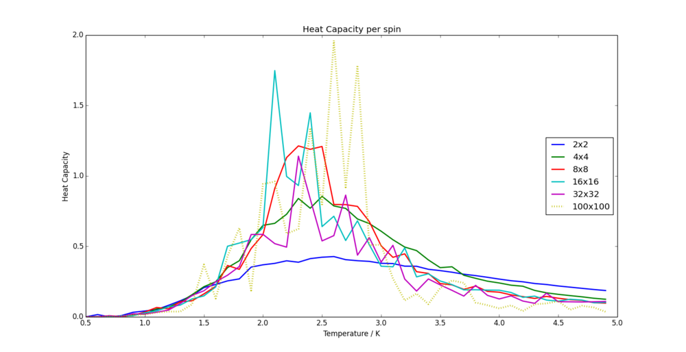
Script used : Heat_capacity.py
The heat capacity has a clear peak at the same temperature range over which the phase transition occurred, as predicted. This peak makes physical sense, because as the phase transition occurs, the new thermal energy being added to the system is no longer increasing the temperature, but driving the increase in entropy. Thus, it appears that the system has a larger heat capacity at this specific transition temperature. It is also clear that the smaller lattice sizes have a broad hump rather than a peak, and the larger system sizes have sharper peaks (limited by the number of temperature points, however). A trend can also be fairly clearly seen from within the 16, 32 & 100 length lattices, in that the peak appears to be shifted towards higher temperatures for larger lattice sizes.
NJ: The peak actually shifts down in temperature as the lattice size is increased, see your later graphs.
Locating the Curie Temperature
Task 17
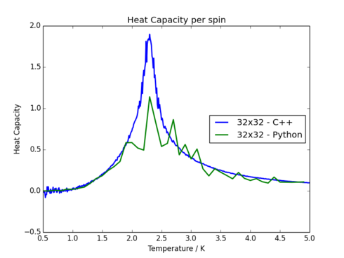
A more thorough set of heat capacity runs using C++ with more temperature points is compared to the results found with Python. A surprisingly good comparison can be found for the smaller lattice sizes, though the results become more disperse for large lattice sizes. The heat capacity Vs. temperature for a 4 by 4 and a 32 by 32 lattice is shown to demonstrate the contrast.
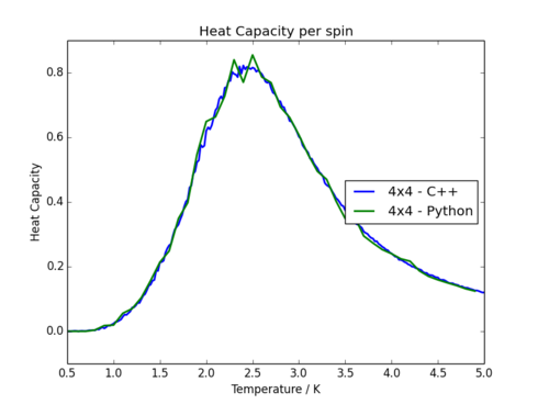
Task 18
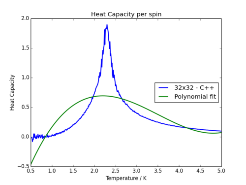
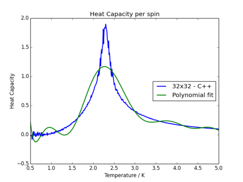
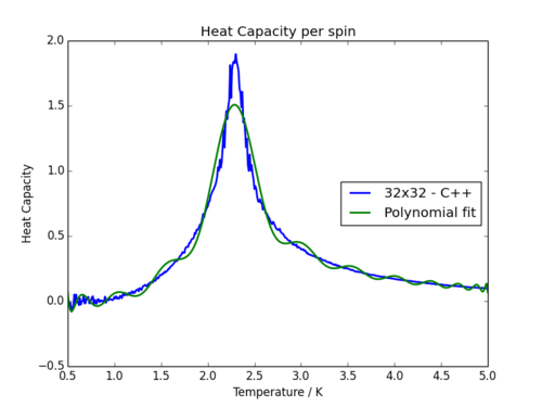
In order to more precisely locate the Curie temperature, the C++ data (much smoother than the Python data) was fitted to a polynomial. This proves quite difficult to find a good match however, since the nature of the peak is very sharp, not indicative of a normal polynomial. As one would expect, fitting to a higher order polynomial produces more accurate results, though it proves impossible to get close to the profile of the heat capacity graphs. Three attempts are shown below which demonstrates the issue:
| Order 3 Polynomial | Order 10 Polynomial | Order 50 Polynomial |
|---|---|---|
|
|
|
NJ: Nice plots
It is visually clear that the 3rd order fit is nowhere near accurate enough to replicate the data, and to have a 50th order polynomial is slightly ridiculous. In order to combat this problem slightly, it makes more sense to simply fit the data around the critical region, since it is only this region containing the Curie temperature in which we are interested.
Task 19
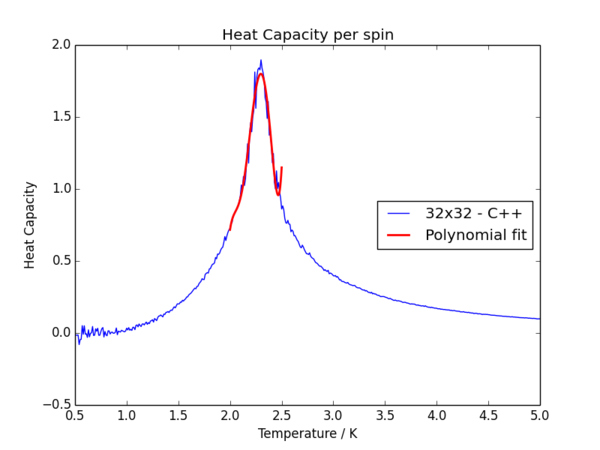
To overcome the problem above, the data was fitted only in the temperature range 2.0 to 2.5 K, with the result on the right. This was again done on the 32 by 32 lattice. This uses a much more manageable and realistic 5th order polynomial, and gives a very good fit to the data.
In order to make the code more compatible with all of the lattice sizes, I took away the manual aspect of choosing the range over which to fit the data, and made it automatic. In this way, the code finds the peak of the C++ data (which is roughly correct with respect to the resulting peak of the polynomial fit), and sets the fitting range from this. The few lines of code controlling this are as follows, adapted from the method of locating the maximum turning point on the fitted polynomial:
T = a[:,0]    #C++ Temperature values
C = a[:,5]    #C++ Heat capacity values

c_data_max = np.max(C)
t_data_max = T[C == c_data_max]
T_min = (t_data_max - 0.2)
T_max = (t_data_max + 0.2)
Task 20
The linear equation can now be used to fit the Curie temperatures of the finite lattice sizes in order to estimate the Curie temperature of an infinite Ising lattice. The equation being , and the linear plot at follows:
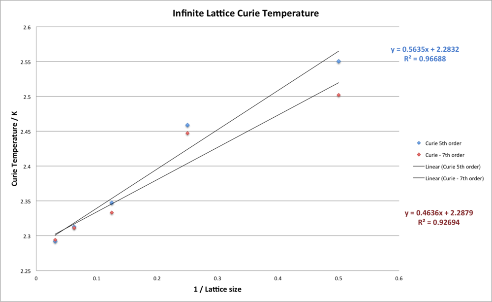
The equation on the graph shows that the intercept corresponding to the Curie temperature for an infinite Ising lattice is 2.283 K. The point corresponding to the 4 side lattice appears to be slightly off, which is reasonable given the noise in the data, and the fit is still quite good, with value of 0.967.
However, out of interest, another fit was performed over the 5 lattice sizes, this time using a 7th order polynomial, to see if a more accurate straight line fit can be made. This was chosen because the fit of the 7th order polynomial appeared to more closely recognise the actual peak of the C++ data. Having said this, the results gave a very similar pattern about the straight line, and also a very similar value for the Infinite lattice Curie temperature, 2.288 K.
To validate these calculated values, they are compared to a literature value. In 1941, a method wa develpoed using purely Boltzmann statistics which provides a simple equation which theorised the Curie temperature as 2.269 K.[1] This follows having shown that . [2]
This value is in surprisingly good agreement with the one obtained with the C++ simulations, being only ~ 0.01 K out. However, there is some obvious variation in the value of Curie temperature calculated for each lattice size. Assuming the relationship between finite and infinite lattice Curie temperature is perfectly valid for all sizes, the curie temperature calculated for the 4 side lattice seems off. This source is error is likely to arise due to the very small relative lattices sizes. It is not entirely clear whether the 2 side or 4 side lattice is an outlier, but they probably both have a much larger error than the larger lattice sizes. This is a reasonable assumption, given that the fluctuations in the smaller lattices are bound to appear much more significant in relation to its size. To observe a large scale fluctuation in the distribution of spins during the simulation of a very large lattice is much more unlikely, given its size and the fact that the simple metropolis algorithm only randomly flips spins one at a time.
NJ: Well spotted - it would be better to ignore the very small lattices, and do some simulations with larger lattice sizes.
References
- ↑ H. Kramers and G. Wannier, Phys. Rev., 1941, 60, 252–262. DOI:10.1103/PhysRev.60.252
- ↑ Richard J. Gonsalves URL:http://www.physics.buffalo.edu/phy410-505/2011/topic5/app2/ accessed 2015.02.13

