Talk:Mod:CEW complab 2
JC: General comments: All tasks completed and most answers correct. Try to make your explanations more concise and make sure that you fully understand the background to each task and show this in your answer.
Liquid Simulations
Introduction to molecular dynamics simulation
Numerical Integration
The Verlet algorithm and the modified velocity-Verlet algorithm can be used to numerically calculate the positions of atoms in a molecular dynamics simulation. These numerical methods require the simulation to be discretised into a series of timesteps, rather than treating the atomic positions, velocities and forces as continuous functions of time. The velocity-Verlet algorithm is:
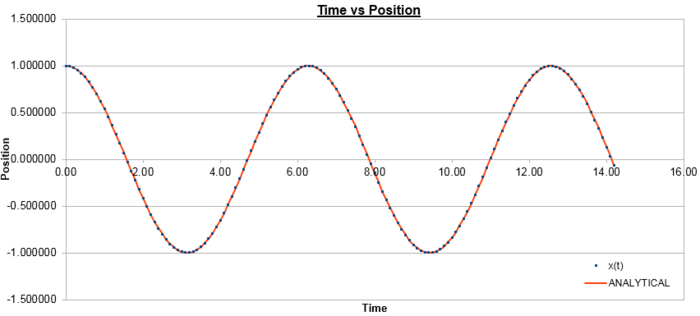
The plot below in figure 1 shows the atomic positions as a function of time as calculated by the velocity-Verlet algorithm, and the classical harmonic oscillator, where:
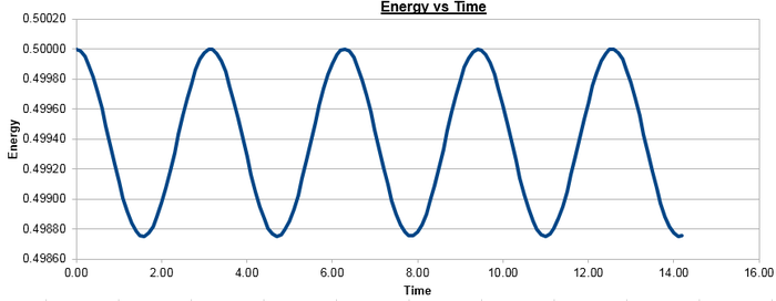
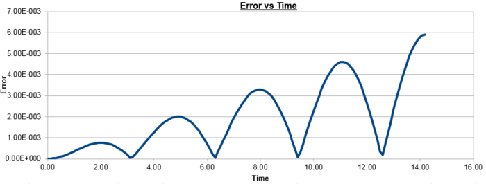
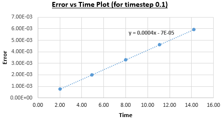
Figure 2 plots the energy as a function of time, which was calculated by summing the kinetic energy term, , and the potential energy term, , and figure 3 plots the error, which was calculated as the difference in the positions found by the velocity-Verlet algorithm and the classical harmonic oscillator, as a function of time. Figure 4 plots the error maxima from figure 3 as a function of time.
The choice of timestep can influence the error of the calculation, as a small timestep is desired to most accurately simulate the system but calculations with a smaller timestep take longer to run than those with a larger timestep. By the harmonic oscillator the total energy should be a constant over the course of the simulation, and it was found that a timestep of is required to ensure the total energy does not change by more than 1% over the course of the simulation. This can be determined by varying the timestep and calculating the size of the fluctuations of the total energy for the simulation, compared to the average constant energy value that would arise from the harmonic oscillator, so monitoring the total energy of of the system when modelling it numerically is important as it allows for the error of the calculation to be determined.
JC: Good choice of timestep.
Atomic Forces
The Lennard-Jones potential describes molecular interactions, and is made up of a repulsive and an attractive part. A Lennard-Jones potential is shown in figure 5 and the equation that governs it is given below:
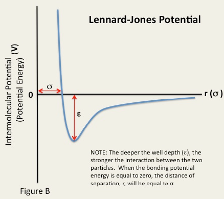
Setting this to zero enables the separation at zero potential, , to be found:
The force is the derivative of the potential with respect to the separation and is shown for the Lennard-Jones potential below:
When the force is given by:
The equilibrium separation,, occurs when the force is zero so is found by:
At the depth of the potential well is given by:
Taking , the integral below can be expressed as:
This result can be used to evaluate the integrals below:
Periodic Boundary Conditions
For simulations, realistic volumes of particles cannot be used as this leads to a huge number of atoms that need to be simulated. This can be shown by considering a system of water molecules:
Taking the concentration of water as , under standard conditions, the number of molecules of water in is the concentration of water multiplied by Avogadro's number ():
The volume of water molecules under standard conditions can be found by dividing the number of water molecules by Avogadro's number to convert to the number of moles of water, and by the concentration of water:
For the simulations run it would not be possible to simulate of water due to the large number of particles, however, applying periodic boundary conditions allows for bulk systems to be simulated with a small system volume. Applying periodic boundary conditions ensures that the number of particles is kept constant, and an example of applying these conditions is described below:
After an atom at position in a cubic simulation box which runs from to has been moved along the vector , it will end up in the position , due to the application of periodic boundary conditions, not outside the simulation box.
Reduced Units
The simulations run are carried out in reduced units. The example for argon below demonstrates how reduced units can be converted into real units:
The Lennard-Jones parameters for argon are , and the cutoff separation is . These values are given in reduced units and can be converted into real units by:
The well depth is given by , so can be found as:
The reduced temperature is , and can be converted into real units by:
JC: All maths and calculations correct and nicely laid out. Give your answers to a consistent number of s.f. though and not more than used in the question.
Equilibration
Creating the simulation box
In these simulations, when particles are too close together they will have a high, repulsive force. Randomly generating the starting coordinates can lead to some atoms being very close to each other, which results in very large repulsive forces between them, and this can cause the calculation to fail due to the size of the force. Instead simulations start from a lattice, which will equilibrate over time. For a simple cubic lattice unit cell with lattice spacing , the number density of lattice points is found by:
For a face centred cubic (FCC) lattice unit cell with the number density of lattice points , the lattice spacing can be found using:
A simulation for the simple cubic lattice with the input file command below leads to the formation of atoms, as there is one atom per unit cell:
create_atoms 1 box
and this is acknowledged in the ouput file by the line:
Created 1000 atoms
For an FCC lattice the input command would lead to the formation of atoms, as there are four atoms per unit cell in the FCC lattice.
Setting the properties of the atoms
The properties of the atoms in the simulation are defined by the lines below:
mass 1 1.0
pair_style lj/cut 3.0
pair_coeff * * 1.0 1.0
The first line of the script means the mass of particle is , the second line means the global cutoff for the Lennard-Jones interactions is at a distance of , and the third line means the pairwise force field coefficients for all atoms, from atoms to , are and . For these simulations the velocity-verlet algorithm is being used, as and have been specified.
JC: Why is a cutoff used with the Lennard-Jones potential? For the Lennard-Jones potential, the pairwise coefficients are epsilon and sigma.
Running the simulation
The lines from an input file below:
 ### SPECIFY TIMESTEP ###
 variable timestep equal 0.001
 variable n_steps equal floor(100/${timestep})
 variable n_steps equal floor(100/0.001)
 timestep ${timestep}
 timestep 0.001

 ### RUN SIMULATION ###
 run ${n_steps}
 run 100000
could be replaced by:
 timestep 0.001
 run 100000
The advantages of the first method are that a variable "timestep" is defined, so every time:
${timestep}
is used in the input file, the amount defined by the line:
variable timestep equal 0.001
is used. This means the simulation will run for the same amount of time, irrespective of the timestep used as the variable "n_steps" is defined as:
variable n_steps equal floor (100/${timestep})
and this value is then used to determine the number of timesteps the simulation is run for in the line:
run ${n_steps}
Using the second method would require the number of timesteps needed to a run a simulation of a certain length to be calculated manually for each timestep used, which would take longer and could lead to errors.
JC: Good understanding.
Checking equilibration
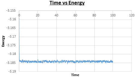
It is important to check that the system reaches equilibrium over the course of the simulation. For the experiment with the timestep the simulation does reach equilibrium, at time , as can be seen in Figures 6, 7, and 8. Figure 9 shows a plot of the energy of all five of the experiments, which were each run with a different timestep. It can be seen that the experiment run with timestep gave a very poor result, as the energy does not reach equilibrium. The largest timestep used to give a useful result is as it reaches equilibrium. However, for timesteps above the energy is dependent on the timestep chosen, which is seen by the energies averaging at increasingly higher values for timesteps and , so the timestep has been chosen to carry out further calculations.
 |
 |
| Figure 6: Plot of time vs energy. | Figure 7: Plot of time vs temperature. |
 |
 |
| Figure 8: Plot of time vs pressure. | Figure 9: Plot of time vs energy for all of the timesteps. |
JC: Good choice of timestep and clear justification.
Running simulations under specific conditions
Thermostats and Barostats
is a constant factor that is required to keep the instantaneous temperature, , and the target temperature, , equal. This is required to ensure the kinetic energy of the system remains at the correct value. It can be found using equipartition theory, where each degree of freedom contributes , on average, to the energy. This gives equations one and two, which are divided by each other to give in terms of and .
Equation one:
Equation two:
JC: Correct derivation.
Examining the Input Script
The input script below describes how average values will be determined.
### MEASURE SYSTEM STATE ###
thermo_style custom step etotal temp press density
variable dens equal density
variable dens2 equal density*density
variable temp equal temp
variable temp2 equal temp*temp
variable press equal press
variable press2 equal press*press
fix aves all ave/time 100 1000 100000 v_dens v_temp v_press v_dens2 v_temp2 v_press2
run 100000
IN the penultimate line,
is the how often input values will be taken,
is the number of times to use input values for calculating averages, and
is how often averages are calculated. In this case averages will be calculated every
timesteps, using
measurements from the simulation, which are found by sampling the values every
timesteps before the average is calculated. The final line is the number of timesteps that the simulation will run for, so in this case
timesteps of
will be carried out, so the simulation will run for time
.
JC: Good understanding.
Temperature and Pressure Control
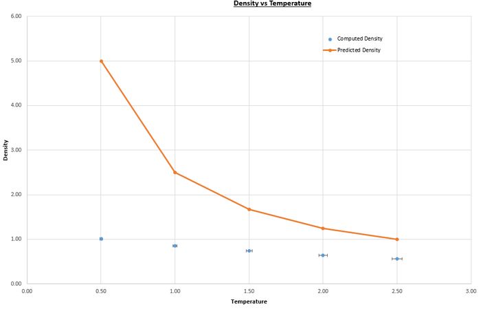
Simulations using the velocity-Verlet algorithm on the Lennard-Jones system were carried out at pressures and , and temperatures , , , and (values in reduced units), with timestep . The pressures and temperatures were chosen as they are close to the equilibrium values that were previously calculated, and the timestep was chosen at it was the largest that gave valid results. The plots in figures 10 and 11show both the computed values for the density using the velocity-Verlet algorithm and the predicted values, found using the perfect gas law with as the simulations are run in reduced units:
 |
 |
| Figure 10: Plot of density versus temperature for pressure. | Figure 11: Plot of density vs temperature for pressure. |
JC: Joining up the ideal gas data points using straight lines is misleading as you know that the ideal gas law doesn't follow these lines. Why do the simulation and ideal gas results get closer together as temperature increases?
The perfect gas law assumes that the volume of the particles is negligible and that there are no intermolecular interactions between the particles, so is best applied to dilute gas systems. The difference between the computed and predicted values increases with pressure because the system becomes less dilute, so less ideal. The computed values are higher than the predicted values as they were found considering intermolecular interactions, as is instructed in the script by the lines below (purpose of commands discussed previously):
pair_style lj/cut/opt 3.0
pair_coeff 1 1 1.0 1.0
JC: Good understanding.
Calculating heat capacities using statistical physics
The heat capacity of a system is the amount of energy needed to increase the temperature of the system by , so is a measure of the amount of thermal energy that can be absorbed. Generally this increases with temperature, as more degrees of freedom are possible (rotational and electronic, in addition to translational) so the system can absorb more thermal energy, but for these simulations the particles are taken as hard spheres so no rotations are possible, and since the simulations are classical no electronic transitions are considered. In the canonical ensemble (NVT) the heat capacity can be calculated using:
The heat capacity was found using this equation for simulations of a Lennard-Jones system, with densities and , at temperatures of , , , and (all values in reduced units), with timestep . Figure 12 shows plots of heat capacity over volume vs temperature for each of the densities.
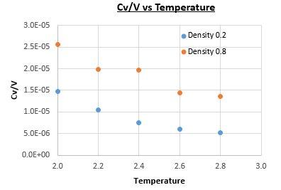
The plot in Figure 12 doesn't follow the expected increasing heat capacity with temperature, but instead the heat capacity decreases with temperature. This can be explained by considering that, at higher energies, the energy levels are closer together so for a given energy level there is a higher degeneracy. This means that in order to achieve a specific population of energy levels at a higher temperature, less energy is required than would be needed for the equivalent density of states at a lower temperature. Also, the heat capacity of the system with density is lower than that of the system with density . This is due to there being more particles per unit volume at the higher density, so to increase the temperature by there are more particles to absorb the energy before the temperature of the system is raised, at the higher density.
The input file for this simulation can be seen here: File:Cew 41.in.
JC: Good explanations. More analysis in addition to what is done in this experiment would be needed to explain the trend with temperature in more detail.
Structural properties and the radial distribution function
The solid, liquid and vapour phases of a Lennard-Jones system were simulated using the densities and temperatures given below (in reduced units) [1]:
| Phase | Density | Temperature |
|---|---|---|
| Solid | 1.20 | 1.40 |
| Liquid | 0.80 | 1.20 |
| Vapour | 0.01 | 1.11 |
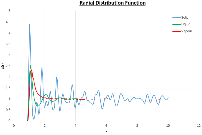
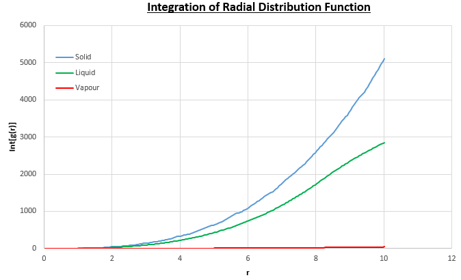
The plots of the radial distribution function (RDF) and its integral from these simulations are shown in figures 13 and 14.
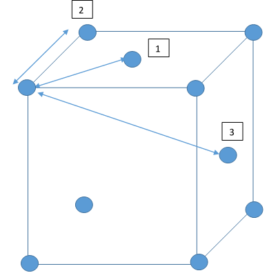
The peaks in the RDFs (figure 13) correspond to the nearest neighbours, so the RDF for the solid phase Lennard-Jones system has many clear peaks. However, those for the liquid and vapour phases do not due to the absence of long range order so the peaks become too small to be observed as the distance between nearest neighbour is too long. For the solid phase, the first three peaks in the RDF correspond to the first three nearest neighbours, which are illustrated in figure 15. The coordination numbers for these peaks can be found by comparing the peak positions in the RDF and the integration of the RDF (figure 14) at the at these positions. This analysis gives the coordination numbers , and for the first, second and third peaks respectively. The lattice spacing, , can be determined using trigonometry from the first nearest neighbour separation, (determined from figure 13):
JC: The lack of peaks at large distances (r) in the liquid and vapour RDFs is due to a lack of long range order in these phases, not due to large distances between nearest neighbours. How can you have fractional coordination numbers?
Alternatively the lattice spacing can be taken as the distance to the second nearest neighbour, which results in a lattice spacing of . This is good agreement with the calculated result above.
JC: Good idea to compare the lattice parameter calculated from the first and second peaks.
Dynamical properties and the diffusion coefficient
Mean Squared Displacement
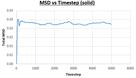
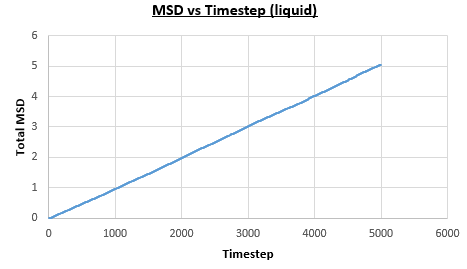
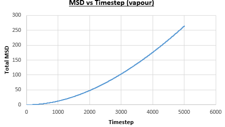
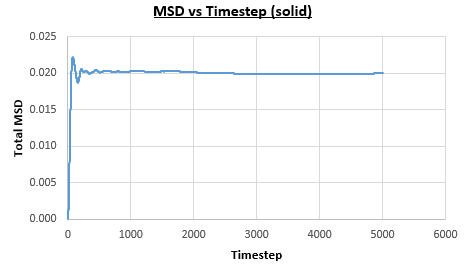
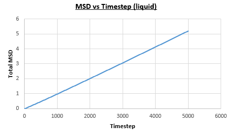
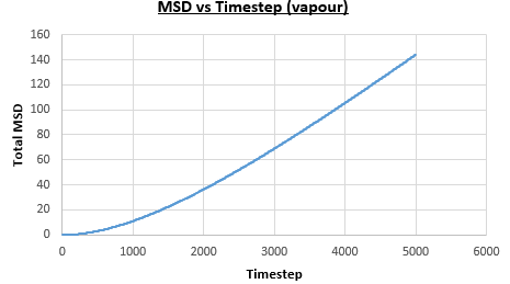
The solid, liquid and vapour phases of a Lennard-Jones system were simulated using the densities and temperatures used previously given, and timestep . From these simulations the mean squared displacement (MSD) was calculated. Figures 16 to 21 below show plots of the MSD vs the timestep for a Lennard-Jones solid, liquid and gas system, with and atoms. The gradient of the line increases on moving from the solid to the liquid to the vapour phase, which was expected, as the atoms are able to move most easily in the vapour phase, so will have a greater MSD.
The diffusion coefficient can be found from the mean squared displacement by the equation below:
The gradient of the line, once it has established linear behaviour, can be taken and converted to a function of time (instead of timestep) by dividing the gradient by the timestep, . This can then be divided by to give the diffusion coefficient. The results are summarised below:
| Type of System | with atoms | with atoms |
|---|---|---|
| Lennard-Jones Solid | Gradient, | Gradient, |
| Lennard-Jones Liquid | Gradient, | Gradient, |
| Lennard-Jones Vapour | Gradient, | Gradient, |
JC: Give answers to 3 s.f. rather than 3 d.p. and show the lines of best fit used to calculate the diffusion coefficients on the graphs.
Velocity Autocorrelation Function
The velocity autocorrelation function (VACF), given by , is another method that can be used to calculate the diffusion coefficient, as:
The VACF can be found by evaluating :
For the 1D harmonic oscillator:
and
The VACF for the 1D harmonic oscillator can be evaluated to give the result shown below:
(, )
JC: Derivation is correct, but you should explain in the last step that the second term must be zero as it is an integral of an odd function with limits equally spaced about zero.
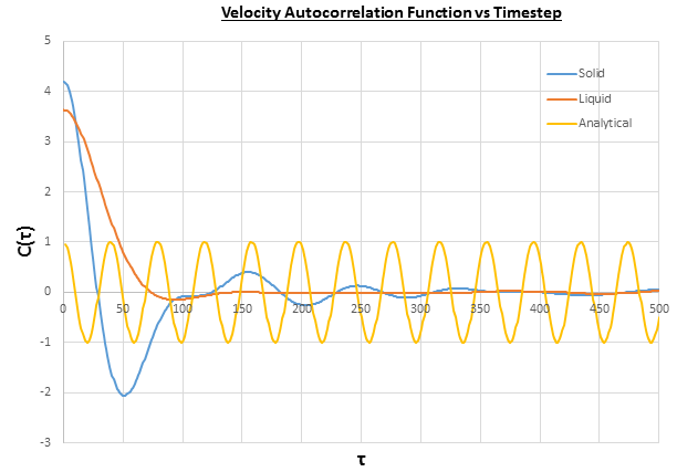
Figure 22 shows the VACF for a Lennard-Jones solid and liquid with atoms, which both show fluctuations due to changes in velocity of the particles. These are caused by collisions with other particles in the system, which cause a change in the direction of the motion of the particle, hence the change in velocity. The differences between the fluctuations observed in the solid and liquid VACFs is due to the distances between the particles, so in the solid the particles are closer together so collide more frequently than in the liquid, which leads to more fluctuations in the VACF for the solid. Furthermore, for both the solid and liquid the VACF decays to zero, as the energy of the particles is dispersed randomly throughout the system upon collisions between particles. The differences between the harmonic oscillator VACF ("analytical") and the Lennard-Jones solid and liquid system are that there are regular fluctuations in the harmonic oscillator, and that the system doesn't decay to zero. The regular fluctuations are caused by changes of velocity each time the spring reaches its fully extended state, as is governed by Hooke's law:
The system doesn't decay to zero because there are no collisions in the harmonic oscillator, so the energy of the particles remains constant and isn't randomly dispersed among the particles.
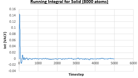
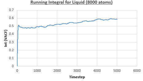
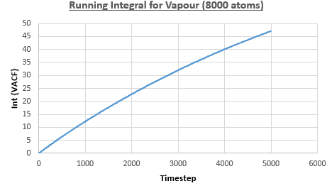
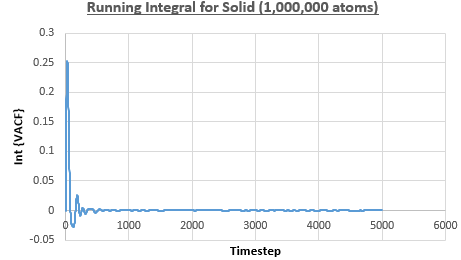
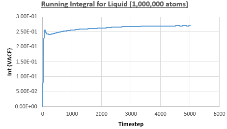
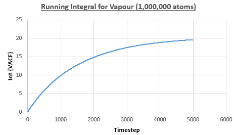
The integral under the VACF can be estimated using the trapezium rule, and this can be used to estimate the diffusion coefficient, as described above. Figures 23, 24 and 25 show the running integrals for each of the Lennard-Jones solid, liquid and vapour phases with atoms and figures 26, 27 and 28 show the running integrals for them with atoms. The running integrals for the solid systems show that the VACF reaches equilibrium, where the gradient decreases to close to zero. This is also true for the liquid simulation with atoms, but not for the other simulations of the liquid and vapour phases. The solid reaches equilibrium the most rapidly as the atoms are able to move the least, but this occurs most slowly in the vapour systems as the particles have more energy so are able to move around more rapidly. This means it takes a longer amount of time for the velocities to reach an average, equilibrium value.
For the Lennard-Jones solid, liquid and vapour, with and atoms, the diffusion coefficients were predicted by the method described above to give the results in the table below. The largest source of error in the estimates of the diffusion coefficient from the VACF is that it is impossible to calculate the integral for infinite time, so this introduces error into calculating the diffusion coefficient, especially when the system doesn't reach an equilibrium state.
| Type of System | with atoms | with atoms |
|---|---|---|
| Lennard-Jones Solid | ||
| Lennard-Jones Liquid | ||
| Lennard-Jones Vapour |
JC: Can you compare the diffusion coefficients calculated from the MSD with those calculated from the VACF?
Summary
Molecular dynamics simulations can be used to determine a lot of thermodynamic data about a system, and good agreement of simulated data and classically calculated data is seen. However, it is important to note that error can arise due to simulations being run with a small number of atoms, and over a limited period of time.
