Talk:Mod:CENPYTHON

Note: In the following context, energy, magnetisation and heat capacity are all reduced quantities and they are in the units of k_BT, reduced Plank constant and k_B, respectively. However temperatures are measured in J/k_B, where J is a constant measure how strong the interaction is between the spin.

Introduction to the Ising Model

TASK1

Show that the lowest possible energy for the Ising model is $E = - D N J$ , where $D$ is the number of dimensions and $N$ is the total number of spins. What is the multiplicity of this state? Calculate its entropy.

Answer:

In one dimensional model, each spin is adjacent to 2 spins; and for the two dimensional model, each spin is adjacent to 4 spins; as for the three dimensional model each spin is adjacent to 6 spins. Therefore there are total number of $2 D$ interactions for one spin in a system with dimension of $D$ .Since the lowest energy configuration is when the maganetic moment parallel to each other, the lowest interaction energy = $2 D (- \frac{1}{2} J s_{i} s_{j})$ where $s_{i} s_{j}$ = 1. Therefore for a system with $N$ spins, the lowest possible energy = $N 2 D (- \frac{1}{2} J \times 1)$ = $- N D J$ .

The two parallel spins can be either both upwards or both downwards, therefore the multiplicity of this state is equal to 2. The entropy S=K_BlnW = K_Bln 2=9.57x10^-24JK^-1.

NJ: Nice explanation.

TASK2

Imagine that the system is in the lowest energy configuration. To move to a different state, one of the spins must spontaneously change direction ("flip"). What is the change in energy if this happens ( $D = 3, N = 1000$ )? How much entropy does the system gain by doing so?

Answer:

1. When one of the spin change its direction, there will be 6 new distinct interactions with each s_is_j = -1. Whereas the original interactions have s_is_j = 1. Therefore the change in energy = 6J - (-6J) = 12J.

2. Since N = 1000, and the spin can either be from up to down or down to up. Therefore S = K_Bln2000, and the ΔS= K_Bln2000 - K_Bln2 = K_Bln1000=9.53X10^-23.

NJ: correct

TASK3

Calculate the magnetisation of the 1D and 2D lattices in figure 1. What magnetisation would you expect to observe for an Ising lattice with $D = 3, N = 1000$ at absolute zero?

Answer:

1. For 1D, M = 1; for 2D, M = 1.

2. M = ±1000

NJ: good! A quick comment about how you know the answer to part 2 would be good.

Calculating the energy and magnetisation

In this section, two functions energy() and magnetisation() in file IsingLattice.py were completed which can be used to calculate energy and magnetisation for a given lattice.

TASK

NJ: Where is the code for the original version of your energy() and magnetisation() functions?

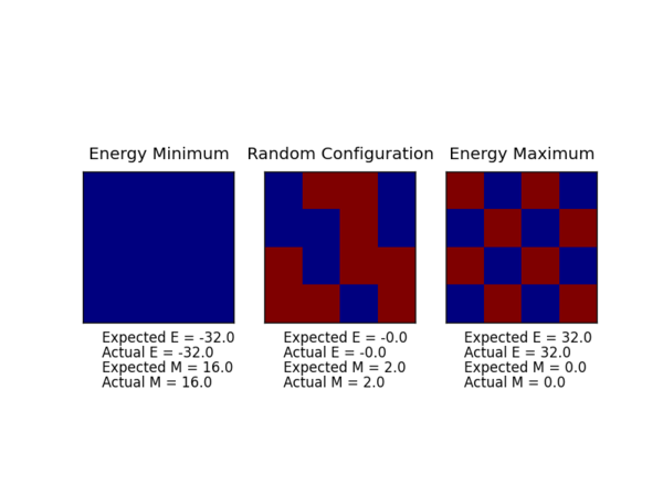
After completing the two functions IsingLattice.py, file ILcheck.py allows us to check whether the two functions are correct or not. The output of ILcheck.py is shown below and indicates the two completed functions are correct.

Introduction to Monte Carlo simulation

In this section, a new function montecarlocycle(T) were completed using the Monte Carlo algorithm to perform a single step simulation. By using the statistic() function average properties such as energy, magnetisation, energy² and magnetisation² are calculated.

TASK1

How many configurations are available to a system with 100 spins? To evaluate these expressions, we have to calculate the energy and magnetisation for each of these configurations, then perform the sum. Let's be very, very, generous, and say that we can analyse $1 \times 1 0^{9}$ configurations per second with our computer. How long will it take to evaluate a single value of ${⟨ M ⟩}_{T}$ ?

Answer

There are 1.27 x 10³⁰ configuration and it will take 1.27 x 10²¹ seconds to complete the calculation, which is equivalent to 4 x 10¹³ years.

NJ: I would have liked to have seen how you arrived at this just writing 2^100 for the answer would have been fine, but good.

TASK2

If $T < T_{C}$ , do you expect a spontaneous magnetisation (i.e. do you expect $⟨ M ⟩ \neq 0$ )? When the state of the simulation appears to stop changing (when you have reached an equilibrium state), use the controls to export the output to PNG and attach this to your report. You should also include the output from your statistics() function.

Answer

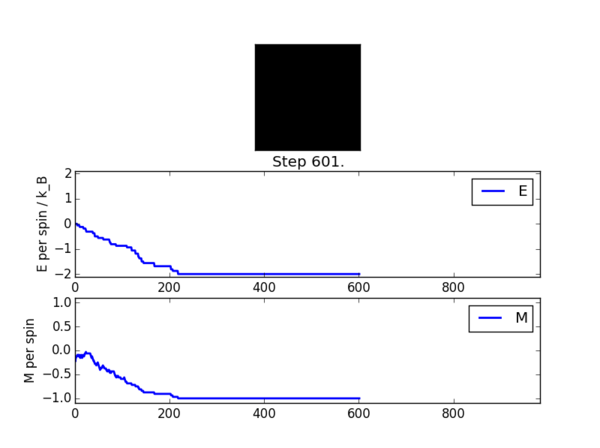
When the temperature is below the Curie temperature, a spontaneous magnetisation is expected as all the spins are highly ordered. Image below shows how a system reach its energy minimum configuration and exhibit a spontaneous magnetization at this energy minimum configuration.

The following quantities are printed after closing the window: $< E >, < E^{2} >, < M >, < M^{2} >$ .

Averaged quantities:
E =  -1.65123581848
E*E =  3.06467154579
M =  -0.854335494327
M*M =  0.801154781199

NJ: In your statistics function, I wouldn't bother defining aveE = 0.0 at the start of the function. It's unnecessary.

Accelerating the code

Numpy functions were used to accelerate the code in the energy() and magnetisation() functions in order to reduce computational time.

TASK1

Use the script ILtimetrial.py to record how long your current version of IsingLattice.py takes to perform 2000 Monte Carlo steps. This will vary, depending on what else the computer happens to be doing, so perform repeats and report the error in your average!

Answer

Total 10 readings were recorded.

%run ILtimetrial.py
Took 7.300468650242022s

%run ILtimetrial.py
Took 7.24796744654293s

%run ILtimetrial.py
Took 7.291973779735898s

%run ILtimetrial.py
Took 7.285238196579542s

%run ILtimetrial.py
Took 7.252695304894331s

%run ILtimetrial.py
Took 7.292496011567579s

%run ILtimetrial.py
Took 7.275512911653763s

%run ILtimetrial.py
Took 7.238346004247262s

%run ILtimetrial.py
Took 7.308245980248785s

%run ILtimetrial.py
Took 7.270112189283395s

%run ILtimetrial.py
Took 7.236859001933453s

Average speed = 7.272440257s

Standard error = 0.008457649

TASK2

Use the script ILtimetrial.py to record how long your new version of IsingLattice.py takes to perform 2000 Monte Carlo steps. This will vary, depending on what else the computer happens to be doing, so perform repeats and report the error in your average!

Answer

After acceleration total 10 readings were recorded.

%run ILtimetrial.py
Took 0.13568766164613066s

%run ILtimetrial.py
Took 0.13802919108715628s

%run ILtimetrial.py
Took 0.15227367127184266s

%run ILtimetrial.py
Took 0.13658750685222287s

%run ILtimetrial.py
Took 0.1391059263605996s

%run ILtimetrial.py
Took 0.15093039345663328s

%run ILtimetrial.py
Took 0.15167296950728826s

%run ILtimetrial.py
Took 0.13515880260516155s

%run ILtimetrial.py
Took 0.14852969941969718s

%run ILtimetrial.py
Took 0.1342230360372696s

%run ILtimetrial.py
Took 0.15064121140113684s

Average speed = 0.142985461s

Standard error = 0.002420864

After acceleration, the new code is 51 times faster than the old code.

NJ: are you surprised by how much faster this makes the code?

The effect of temperature

In this section, energy and magnetisation were monitored at constant temperature which allows us to calculate the number of steps required to reach equilibrium.

TASK1

The script ILfinalframe.py runs for a given number of cycles at a given temperature, then plots a depiction of the final lattice state as well as graphs of the energy and magnetisation as a function of cycle number. This is much quicker than animating every frame! Experiment with different temperature and lattice sizes. How many cycles are typically needed for the system to go from its random starting position to the equilibrium state? Modify your statistics() and montecarlostep() functions so that the first N cycles of the simulation are ignored when calculating the averages. You should state in your report what period you chose to ignore, and include graphs from ILfinalframe.py to illustrate your motivation in choosing this figure.

Answer

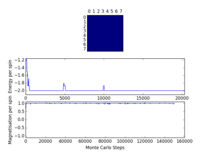
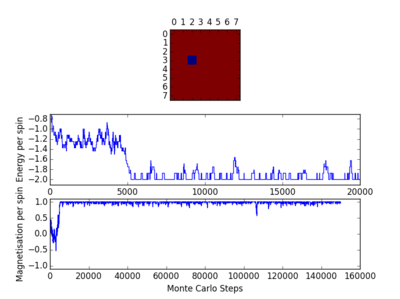
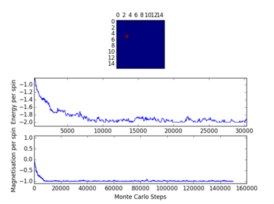
The relaxation steps that the system used to reach equilibrium need to be excluded when calculating the average properties. The steps that need to be excluded for different lattice sizes are shown below. For a 8x8 system, only the first 5000 steps require to be ignored. Whereas for a bigger system such as 16x16, the first 20000 steps need to be excluded. As shown below, as the temperature increases the fluctuation about the equilibrium value increases. However, with a larger lattice, the effect of temperature is less pronounced.

NJ: That's not quite true! It's just that you're plotting E/N, and N is increasing.


	Condition 1	Condition 2
Size	8x8	8x8
Temperature	1	1.5
Period to ignore	500	5000

	Condition 3	Condition 4
Size	16x16	16x16
Temperature	1	2
Period to ignore	9000	20000

TASK2

Use ILtemperaturerange.py to plot the average energy and magnetisation for each temperature, with error bars, for an $8 \times 8$ lattice. Use your initution and results from the script ILfinalframe.py to estimate how many cycles each simulation should be. The temperature range 0.25 to 5.0 is sufficient. Use as many temperature points as you feel necessary to illustrate the trend, but do not use a temperature spacing larger than 0.5. T NumPy function savetxt() stores your array of output data on disk — you will need it later. Save the file as 8x8.dat so that you know which lattice size it came from.

Answer

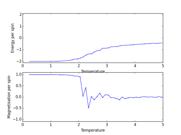
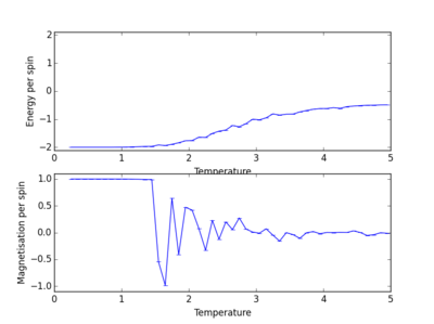
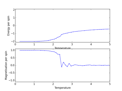
The temperature range is from 0.25 to 5.0 and the temperature spacing = 0.1. For a 8x8 lattice, the first 5000 steps were chosen to ignore and the runtime = 50000. These numbers were deducted based on the analysis of the output from ILfinalframe.py, and the average energy and magnetisation against temperature were plotted and shown below.

The effect of system size

In this section, energy and magnetisation were monitored over a range of temperature in order to study the effect of system size. Some steps were ignored in the calculation, in order to improve the accuracy of the average properties.

TASK1

Repeat the final task of the previous section for the following lattice sizes: 2x2, 4x4, 8x8, 16x16, 32x32. Make sure that you name each datafile that your produce after the corresponding lattice size! Write a Python script to make a plot showing the energy per spin versus temperature for each of your lattice sizes. Hint: the NumPy loadtxt function is the reverse of the savetxt function, and can be used to read your previously saved files into the script. Repeat this for the magnetisation. As before, use the plot controls to save your a PNG image of your plot and attach this to the report. How big a lattice do you think is big enough to capture the long range fluctuations?

Answer

The number of excluded steps and runtime for different lattice sizes are summarised in the table below.


Size	2x2	4x4	8x8	16x16	32x32
number of steps ignored	200	800	5000	20000	90000
runtime	10000	20000	50000	150000	300000
effective runtime per spin	2450	1200	703	508	205

The plots of energy and magnetisation per spin against temperature for each lattice sizes are shown below. The plots of 8x8 lattice is shown in the section above.


Size	2x2	4x4

Size	16x16	32x32

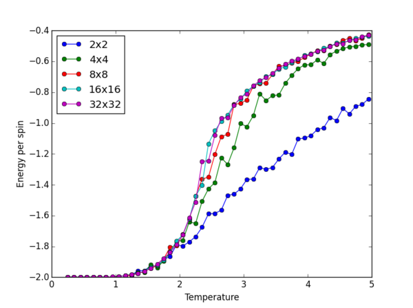
Energy and magnetisation against temperature are plotted below. As we can see from both of the graphs, there is no significant improvement on the quality of the graphs by increasing the lattice size from 16x16 to 32x32. However, the calculation for 32x32 lattice is more computationally expensive than 16x16, therefore 16x16 lattice size is sufficient to monitor the long range fluctuation as a result of a compromise between computational time and accuracy.

NJ: you can probably even get away with using an 8x8 lattice, but good reasoning.

Determining the heat capacity

Heat capacity was calculated from energy for different lattices in order to study the effect of size.

TASK

Write a Python script to make a plot showing the heat capacity versus temperature for each of your lattice sizes from the previous section. You may need to do some research to recall the connection between the variance of a variable, $V a r [X]$ , the mean of its square $⟨ X^{2} ⟩$ , and its squared mean ${⟨ X ⟩}^{2}$ . You may find that the data around the peak is very noisy — this is normal, and is a result of being in the critical region. As before, use the plot controls to save your a PNG image of your plot and attach this to the report.

Answer

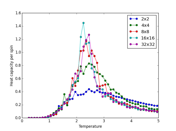
The peak maximum should increase with lattice size as for infinite lattice, heat capacity diverges at the phase transition temperature, i.e. Curie Temperature. Moreover according to $T_{C, L} = \frac{A}{L} + T_{C, \infty}$ , as the lattice size increases, $T_{C, L}$ should decreases because $T_{C, \infty}$ is a constant. Therefore the position of the peak in the graph below should shift to the left with increasing lattice size. However the 32x32 lattice doesn't fit in the trend described above, this is probably due to the small effective runtime per spin (205, calculated in the section above).

NJ: I would put a note in your source code to the effect that the heat capacity calculated is per spin, but this is good otherwise.

Locating the Curie temperature

In this section, the heat capacity values calculated from the Python data were compared to the values obtained from the C++ datat. Then, the C++ heat capacity against temperature curves were fitted using polynomial function in all range and selected range. By doing so, the temperature (Tmax) is obtained at which the heat capacity is at maximum. Tmax was then plotted against 1/L in order to extrapolate the Tmax for infinite lattice.

TASK1

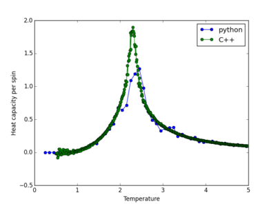
A C++ program has been used to run some much longer simulations than would be possible on the college computers in Python. You can view its source code here if you are interested. Each file contains five columns: $T, E, E^{2}, M, M^{2}, C_{V}$ , and you can read them with the NumPy loadtxt function as before. For each lattice size, plot the C++ data against your data. For one lattice size, save a PNG of this comparison and add it to your report — add a legend to the graph to label which is which. To do this, you will need to pass the label="..." keyword to the plot function, then call the legend() function of the axis object (documentation here).

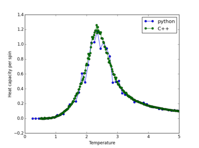
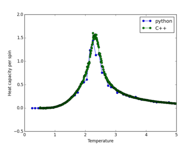
Graphs of heat capacity against temperature of different lattice sizes calculated using python and C++ are shown below. As we can see, the 32x32 result calculated by python differs the most from the C++ data, this is consistent with the argument made earlier about the accuracy of the 32x32 data.


Size	2x2	4x4

Size	8x8	16x16

Size	32x32

NJ: It would be easier to compare here if one of the datasets plotted with only a line, instead of points, but nice otherwise.

TASK2

write a script to read the data from a particular file, and plot C vs T, as well as a fitted polynomial. Try changing the degree of the polynomial to improve the fit — in general, it might be difficult to get a good fit! Attach a PNG of an example fit to your report.

A 20th order polynomial was used to fit the graph of heat capacity per spin against temperature, which is calculated from a 64x64 lattice using C++. The graph suggests that it is not a very good fit.

NJ: again, comparison would be easier if one of these datasets were just a line

TASK3

Modify your script from the previous section. You should still plot the whole temperature range, but fit the polynomial only to the peak of the heat capacity! You should find it easier to get a good fit when restricted to this region.

Answer

By limiting the temperature from 2 to 2.5, the polynomial only requires 8th order to make a good fit. Therefore restricting the temperature range is essential to capture the main feature of the peak.

NJ: again, comparison would be easier if one of these datasets were just a line

TASK4

Find the temperature at which the maximum in C occurs for each datafile that you were given. Make a text file containing two colums: the lattice side length (2,4,8, etc.), and the temperature at which C is a maximum. This is your estimate of $T_{C}$ for that side length. Make a plot that uses the scaling relation given above to determine $T_{C, \infty}$ . By doing a little research online, you should be able to find the theoretical exact Curie temperature for the infinite 2D Ising lattice. How does your value compare to this? Are you surprised by how good/bad the agreement is? Attach a PNG of this final graph to your report, and discuss briefly what you think the major sources of error are in your estimate.

Answer

Tmax for each lattice size was obtained by extracting data from the polynomial fit to the peak region described earlier. Then by fitting the data to $T_{C, L} = \frac{A}{L} + T_{C, \infty}$ , we obtained $T_{C, \infty}$ . $T_{C, \infty}$ = 2.28128933124K. This is relatively close to the theoretical Curie temperature, 2.269K of a infinite 2 dimensional Ising lattice.^[1] There are three major source of errors.

NJ: careful, it's not 2.269K - it's $2.269 J / k_{B}$

Firstly, different temperature range will affect the polynomial fit and therefore give a different Tmax for each lattice. This can greatly affects the position of data point shown in the figure below and in turn the gradient and y intercept of the fitted line.

Secondly, as we can see from the graph, the data points are concentrated at the bottom left corner, this is because we are plotting Tmax against 1/L. In fact there is no way increase the number of data points towards the upper right corner as L can only be integers. However, we can slightly improve the the accuracy of the linear fit by including the 3x3 and 5x5 lattice sizes data.

Finally, the data points of 2x2 and 4x4 lattices are less accurate compare to the larger lattice as the possible energy levels are very limited.

NJ: so do you think including 3x3 and 5x5 would help? What about ignoring the 2x2 and 4x4 points?

Reference

↑ H.A. Kramers and G.H. Wannier, Phys. Rev. 60, 252 (1941)

[Curie_temperature-1] H.A. Kramers and G.H. Wannier, Phys. Rev. 60, 252 (1941)

[1]