Talk:Mod:ASP9395

JC: General comments: Excellent report, all sections were answered very thoroughly with a lot of extra relevant detail. Explanations were well written, clear and focused, well done.

First Simulation

Simple Harmonic Oscillator

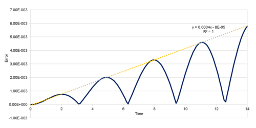
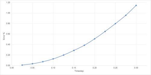
In order to demonstrate a simple molecular simulation, a model classical harmonic oscillator was established. The velocity-Verlot algorithm was used to determine velocity, and kinetic and potential energy was evaluated at each timestep. Variation in total energy was measured for a number of different timesteps (Figures 1-2); total energy must remain approximately constant within a model system to ensure it can realistically simulate a physical system constrained by conservation of energy. Timesteps greater than 0.28 exceed a 1% deviation in energy, and ideally would not be used in such a simulation.

Figure 1: Error in energy for simple harmonic oscillator, with linear fit of position of maxima.

Figure 2: Percentage error in energy for simulations of different timesteps.

JC: Why does the error oscillate over time? Good, thorough analysis of the effect of timestep on total energy.

Lennard-Jones Potential

For a Lennard-Jones interaction, the distance at which no potential energy is present (r₀) was calculated as such:

$\varphi (r)=4ϵ(\frac{{\sigma }^{12}}{r^{12}}-\frac{{\sigma }^6}{r^6})$

$\varphi (r)=0⟹(\frac{{\sigma }^{12}}{r_0^{12}}-\frac{{\sigma }^6}{r_0^6})=0⟹r_0=\sigma$

The distance at which no force is acting upon the atoms (r_eq) was similarly calculated:

$F(r)=-\frac{d\varphi (r)}{dr}=24ϵ(\frac{2{\sigma }^{12}}{r^{13}}-\frac{{\sigma }^6}{r^7})$

$F(r_0)=-\frac{d\varphi (r)}{dr}=24ϵ(\frac{2}{\sigma }-\frac{1}{\sigma })=\frac{24ϵ}{\sigma }$

$F(r_{eq})=0=(\frac{2{\sigma }^{12}}{r_{eq}^{13}}-\frac{{\sigma }^6}{r_{eq}^7})⟹\frac{2{\sigma }^{12}}{r_{eq}^{13}}=\frac{{\sigma }^6}{r_{eq}^7}⟹2{\sigma }^6=r_{eq}^6⟹r_{eq}=(2\sigma {)}^{\frac{1}{6}}$

To model Lennard-Jones interactions across infinite distances, approximations must be made. One such approximation is that interactions between atoms beyond a certain separation are so small as to be ignored. The separation of 3σ is used throughout these simulations; the following calculations demonstrate the steep droppoff rate associated with such forces that justifies this arbitrary cutoff point.

$4ϵ\int \frac{{\sigma }^{12}}{r^{12}}-\frac{{\sigma }^6}{r^6}dr$

$=4ϵ[\frac{{\sigma }^6}{5r^5}-\frac{{\sigma }^{12}}{11r^{11}}]+cst$

When σ = ɛ = 1

$\underset{2\sigma }{\overset{\mathrm{\infty }}{\int }}=4[\frac{1}{5r^5}-\frac{1}{11r^{11}}{]}_2^{\mathrm{\infty }}=4(\frac{1}{11\times 2^{11}}-\frac{1}{5\times 2^5})=-0.0248$

$\underset{2.5\sigma }{\overset{\mathrm{\infty }}{\int }}=4[\frac{1}{5r^5}-\frac{1}{11r^{11}}{]}_{2.5}^{\mathrm{\infty }}=4(\frac{1}{11\times 2.5^{11}}-\frac{1}{5\times 2.5^5})=-0.0082$

$\underset{3\sigma }{\overset{\mathrm{\infty }}{\int }}=4[\frac{1}{5r^5}-\frac{1}{11r^{11}}{]}_3^{\mathrm{\infty }}=4(\frac{1}{11\times 3^{11}}-\frac{1}{5\times 3^5})=-0.0033$

This fast decay of force with distance justifies the LJ cutoff of 3σ; beyond this distance atoms have little interaction with one another and can be approximated as being independent of each other.

JC: All correct, except for r_eq sigma shouldn't be raised to the power 1/6. Good explanation of the integrals.

Scale of Simulation

The volumes that can be simulated in such a way are very limited.

1 mL water = 1 g

1 mol water = 18 g

1 mol = 6.022*10²³ atoms

1 mL water = 6.022*10²³/18 atoms = 3.346*10²² atoms

$\frac{10000}{3.346\times 10^{22}}=2.989\times 10^{-19}\mathrm{m}\mathrm{L}$

A simulation involving 10000 atoms of water only simulates 2.989*10^-19 cm³. This demonstrates the difficulty in modelling large amounts of atoms computationally.

JC: Correct.

Periodic Boundary Conditions

Figure 3a: Diagram depicting periodic boundaries. Boundary conditions are established such that when a particle leaves through one wall, it re-enters through the opposite wall with the same momentum (Figure 3). An atom starting at (0.5, 0.5, 0.5) and moving with vector <0.7, 0.6, 0.2> finishes at what would have been position (1.2, 1.1, 0.7), but with these boundary conditions it can instead be said to finish at (1.2 mod 1, 1.1 mod 1, 0.7 mod 1) = (0.2, 0.1, 0.7). This allows a large volume system to be simulated using minimal processing power; as described above, simulating individual molecules can only provide a very small scale system.

Figure 3b: Animation depicting movement through boundary.

JC: Good explanation and diagram. Periodic boundary conditions remove interfacial effects which would otherwise dominate the behaviour of the simulated system.

Reduced Units

In order to simplify the calculations involved in these simulations, reduced units are used:

Distance $r^{*}=\frac{r}{\sigma }$

Energy $E^{*}=\frac{E}{ϵ}$

Temperature $T^{*}=\frac{k_{B}T}{ϵ}$

Time $t^{*}=\frac{t}{\sigma (\frac{m}{ϵ}{)}^{\frac{1}{2}}}$

In the case of argon, where σ = 0.34nm, ɛ/k_B = 120 K, a distance of 3.2 reduced units corresponds to 1.088 nm, with a well depth of 0.998 kJ/mol. A reduced temperature of 1.5 corresponds to a temperature of 180 °C.

JC: Correct.

Equilibration

Creating the Simulation Box

When creating a simulation of thousands of atoms, they begin in positions pre-determined by a lattice structure. This is to ensure that no two particles are placed in identical or near-identical positions; this would result in an incredibly high potential-energy system, which would result in high kinetic energy and so high temperature.

The number lattice density corresponds to the side length (lattice spacing) as shown in the following equation:

$\text{lattice spacing}=(\frac{\text{density}}{\text{lattice points per unit cell}}{)}^{-\frac{1}{3}}$

Therefore a simple cubic lattice (with one lattice point per unit cell) and a density of 0.8 will have lattice spacing of 1.07722. Similarly, a face-centred cubic with density of 1.2 and 4 lattice points per unit cell will have a side length of 1.49380 reduced units.

When filling a box of 10x10x10 unit cells (volume of 1000 unit cells) with face-centred cubic lattices (which each feature 4 atoms per unit cell) using the create_atoms command, 4000 atoms would be created.

JC: Calculations are correct. Placing two atoms too close together in a starting structure would lead to very high repulsive forces which would make the simulation unstable and cause it to crash.

Interaction Commands

A number of commands are included in the input file to specify the interactions between atoms:

 mass 1 1.0 

The purpose of this command is to specify the relative masses of the atoms used in this system. As only one type of atom was used, only one mass was specified.

 pair_style lj/cut 3.0 

The pair_style command here is used to determine the type of interactions between atoms, and the distance at which atoms stop interacting. In this case, the Lennard-Jones interactions will end at a distance of 3σ.

 pair_coeff * * 1.0 1.0 

This specifies that all pairwise interactions have LJ coefficients σ = 1 and ɛ = 1

Given that $x_i(0)$ and $v_i(0)$ are specified, the integration algorithm used is the velocity-Verlet algorithm.

JC: Correct.

Defining Variables

The input file specifies a number of variables, such as:

 variable timestep equal 0.001 

variable n_steps equal floor(100/${timestep})
timestep ${timestep} 

The purpose of defining these variables is to allow the input file to be easily adjusted. Rather than having to change both lines to specify the new timestep, only the variable timestep equal line needs to be modified, and the other lines will simply read the new timestep value from this line. In more complicated input files, this greatly simplifies the process of changing timestep.

JC: Good explanation.

Choice of Timestep

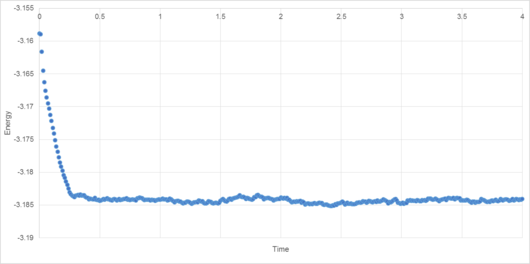
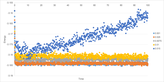
A number of simulations with differing timesteps were created, and their energy, temperature and pressure monitored (Figures 4-7).

Figure 4: Energy change with time for 0.001 timestep simulation.	Figure 5: Temperature change with time for 0.001 timestep simulation.
Figure 6: Pressure change with time for 0.001 timestep simulation.	Figure 7: Convergence of energy over time for five different timestep simulations.

This serves to highlight the two competing factors of any simulation: accuracy of results and time taken to perform. Clearly, a lower variation of energy, temperature and pressure are achieved using a smaller timestep, (Figure 7). However, the smaller the timestep, the greater the time required to run the simulation.

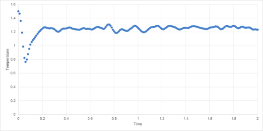
For the 0.001 timestep, the system reaches equilibrium at approximately 0.28 reduced time units (6.06*10^-13 s). The energy associated with the simulation with the smallest timestep, 0.001, converges sharply to -3.184 reduced energy units. The 0.0025 timestep simulation converges to roughly the same energy (also -3.184 to 3 d.p.), but has greater variance. Greater timesteps cause average energy to increase, variance to increase, and in the case of the 0.015 timestep, the energy actually diverges (causing the simulation to become less reliable over time). This timestep therefore cannot be used in a simulation to determine the physical properties of a system.

A timestep of 0.0025 can be used as a compromise between accuracy and speed, though if time or computational resources are limited then 0.01 is suitable (with an energy value converging to approximately -3.181, representing an error of only 0.1%). For the following simulations, a timestep of 0.0025 was used.

JC: Good choice of timestep. The total energy should be independent of the timestep.

Running Simulations under Specific Conditions

Velocity Correction Coefficient

As a system fluctuates at each timestep, certain variables will need to be kept constant. In order to maintain a constant temperature, a velocity correction coefficient (ɣ) is introduced. By multiplying the velocity by this coefficient at each timestep, constant kinetic energy and therefore temperature can be maintained.

$\frac{1}{2}\sum _i^{}{m}_i{\nu }_i^2=\frac{3}{2}N{k}_{B}T$

${\gamma }^2\frac{1}{2}\sum _i^{}{m}_i{\nu }_i^2=\frac{3}{2}N{k}_B\mathfrak{𝔗}$

${\gamma }^2=\frac{\frac{3}{2}N{k}_B\mathfrak{𝔗}}{\frac{1}{2}\sum _i^{}{m}_i{\nu }_i^2}=\frac{\frac{3}{2}N{k}_B\mathfrak{𝔗}}{\frac{3}{2}N{k}_{B}T}=\frac{\mathfrak{𝔗}}{T}$

$\gamma =\sqrt{\frac{\mathfrak{𝔗}}{T}}$

Where $T$ = instantaneous temperature and $\mathfrak{𝔗}$ = target temperature.

JC: Correct.

The Fix Averages Command

fix aves all ave/time 100 1000 100000 v_dens v_temp v_press v_dens2 v_temp2 v_press2

The "fix ave/time" command refers to which timestep values contribute to the final average. In this case, the average at 100000 timesteps is calculated using the value of the 1000 most recent multiples of 100 timesteps - in effect, every 100th timestep is included. If the input were:

fix aves all ave/time 100 999 100000 v_dens v_temp v_press v_dens2 v_temp2 v_press2

Then the average at 100000 timesteps would contain values from the 200th, 300th, 400th... timesteps, omitting the first 100th.

With a timestep value of 0.0025, and a total of 100000 runs, the amount of time in reduced units being simulated is 250. Using the coefficient values of argon described earlier, in real time this corresponds to 54.1 ns.

JC: Good explanation of the averaging procedure.

Plotting Equations of State

Figure 8: Density change with temperature for two pressures of simulated systems and ideal gases

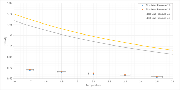
Simulations were run at pressures of 2.6 and 2.8, and temperatures of 1.7, 1.9. 2.1, 2.3 and 2.5 reduced units (Figure 8).

Note that standard deviation in density is too small for the y-axis error bars to be observed at this scale. Reduced units are used throughout to demonstrate relative differences rather than absolute values.

The simulated density is lower than that of an ideal gas at the same conditions. With an equilibrium separation between atoms (r_eq) of 1.122σ and lattice spacing of 1.077σ, the repulsive forces between atoms outweigh the attractive at these inter-atomic distances, causing atoms to spread out from one another and decrease density (compared to the ideal gas, which by definition features no inter-atomic interactions).

Using previously established unit conversion coefficients, the pressures used (2.6 and 2.8 reduced pressure units) can be converted into real units of over 100 MPa, or over 1000 atmospheres. At pressures this high, the ideal gas model also becomes less realistic as interactions between particles become more significant. It is for this reason that at lower pressures the discrepancy between simulated results and the ideal gas law decreases.

JC: Good explanation. How does the discrepancy between simulation and ideal gas results change with temperature?

Heat Capacity

Heat capacities were calculated for two different pressures at a range of temperatures, and these values compared to the National Institute of Standards and Technology Thermophysical Properties of Fluid Systems Database (Figure 9).¹

Figure 9: Volumetric heat capacities at different pressures and temperatures.

Good agreement is found between these values, though a greater level of fluctuation is observed for the higher pressure system.

The volumetric heat capacity was also calculated for each set of conditions (Figure 10):

Figure 10: Volumetric heat capacities divided by total volume at different pressures and temperatures.

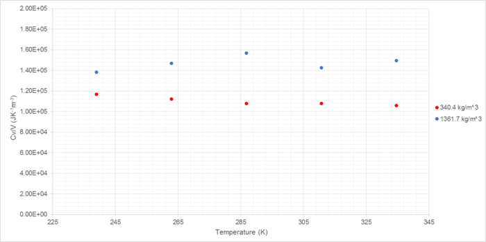Volumetric heat capacity increases with density and shows a slight decrease with temperature. Higher densities have higher heat capacities due to the greater number of atoms within each volume unit; the greater the number of atoms, the more energy must be input in order to cause them all to achieve the required increase in kinetic energy for a given temperature change.

An example input file can be found here.

JC: Great idea to compare heat capacity data to literature values. You could make your script print out the value of the heat capacity directly rather than just calculating the variance in the total energy.

Radial Distribution Function

Solid, Liquid and Gas RDF

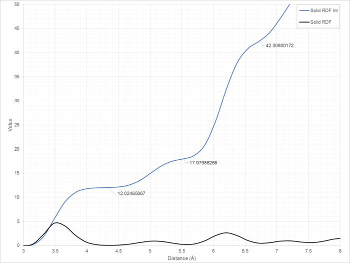
The radial distribution function (RDF) of a system describes the likelihood of finding an atom within a certain separation distance of another. For example, in the case of Figure X, in the solid system, it is almost two times more likely that atoms will have a separation of 3.5 Å than 5.1 Å (Figure 11). These values are normalised, with the average density of atoms in the system equal to one.

RDF converges to unity over very long distances because real systems are not perfectly ordered; knowing the position of one atom does not allow you to accurately predict the position of atoms thousands of angstroms away, and therefore atom density at great distances is equal to average atom density.

Figure 11: RDF versus distance for different phases.

RDF values of liquids converge at a far greater rate than those of solids because they are less structured, and for the same reason, gases converge faster than liquids. The fact that peaks are still visible even at 33 Å implies a very high level of order for the solid structure, due to the restricted freedom of atoms (Figure 21).

Structure of Solid

The first three peaks corresponding to the solid RDF (at distances 3.54, 5.05 and 6.20 Å) have integral values of 12, 6 and 24 respectively (Figure 12). These three peaks correspond to the 12 nearest neighbours, 6 second-closest neighbours and 24 third-closest. These are depicted in Figure 13 as the red, yellow and green atoms respectively (with the central blue atom acting as observer) (Summarised in Table 1).

Figure 12: Use of integrated RDF values to determine coordination number.

Figure 13: Diagram depicting nearest neighbours of an atom in a FCC lattice.

Table 1: Nearest neighbours determined through RDF integration.

Neighbour Proximity	Distance /Lattice Spacing	Distance /Å	Colour	Coordination Number
First	$\frac{\sqrt{2}}{2}$	3.54	Red	12
Second	$1$	5.05	Yellow	6
Third	$\frac{\sqrt{6}}{2}$	6.20	Green	24

One lattice spacing corresponds to 5.05 Å, as determined geometrically using the data in Table 1.

JC: The solid RDF decreases towards 1 at high distances because at these distances there are more possible lattice vectors (possible combinations of unit cell vectors) which are very similar in length. The liquid RDF shows short range solid like ordering, but no long range order. Diagram of lattice very clearly shows all of the atoms responsible for the first 3 peaks in the RDF. Can you calculate the lattice spacing from the first and third peaks as well and check that they agree, or calculate an average value.

Diffusion Coefficient

Mean Squared Displacement

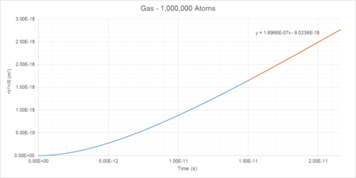
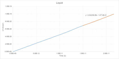
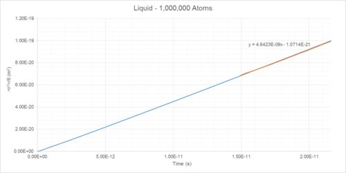
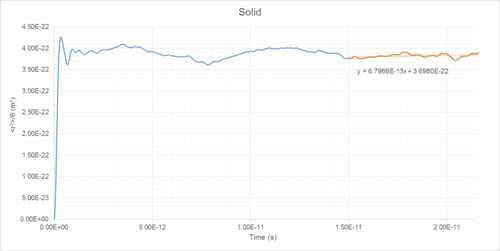
Mean Squared Displacement (MSD) of atoms within a simulated system can be used to determine diffusion coefficient (D) (Table 1). This is a measure of the rate that particles spread out throughout a system (Figures 14-19).

Figure 14: MSD variation with time for a simulated gas.	Figure 15: MSD variation with time for a large-scale simulated gas.
Figure 16: MSD variation with time for a simulated liquid.	Figure 17: MSD variation with time for a large-scale simulated liquid
Figure 18: MSD variation with time for a simulated solid.	Figure 19: MSD variation with time for a large-scale simulated solid.

Velocity Autocorrelation Function (Harmonic Oscillator)

The velocity autocorrelation function (VACF) for a simple harmonic oscillator can be determined as follows:

$x=Acos(\omega t)$

$\frac{dx}{dt}=-A\omega sin(\omega t)=-A\omega sin(\omega t)$

$C_v=\frac{\underset{-\mathrm{\infty }}{\overset{\mathrm{\infty }}{\int }}{A}^2{\omega }^{2}sin(\omega t)sin(\omega t+\omega \tau )dt}{A^2{\omega }^2\underset{-\mathrm{\infty }}{\overset{\mathrm{\infty }}{\int }}si{n}^2(\omega t)dt}$

$sin(\omega t+\omega \tau )=sin(\omega t)cos(\omega \tau )+sin(\omega \tau )cos(\omega t)$

$C_v=\frac{\underset{-\mathrm{\infty }}{\overset{\mathrm{\infty }}{\int }}sin(\omega t)(sin(\omega t)cos(\omega \tau )+sin(\omega \tau )cos(\omega t))dt}{\underset{-\mathrm{\infty }}{\overset{\mathrm{\infty }}{\int }}si{n}^2(\omega t)dt}$

$C_v=\frac{\underset{-\mathrm{\infty }}{\overset{\mathrm{\infty }}{\int }}si{n}^2(\omega t)cos(\omega \tau )+sin(\omega t)cos(\omega t)sin(\omega \tau )dt}{\underset{-\mathrm{\infty }}{\overset{\mathrm{\infty }}{\int }}si{n}^2(\omega t)dt}$

The RHS of the numerator is odd and so equals 0 upon symmetric integration

$C_v=cos(\omega \tau )\frac{\underset{-\mathrm{\infty }}{\overset{\mathrm{\infty }}{\int }}si{n}^2(\omega t)dt}{\underset{-\mathrm{\infty }}{\overset{\mathrm{\infty }}{\int }}si{n}^2(\omega t)dt}=cos(\omega \tau )$

JC: Correct.

Velocity Autocorrelation Function (Simulation Data)

Figure 20: VACF for liquids, solids and SHO.

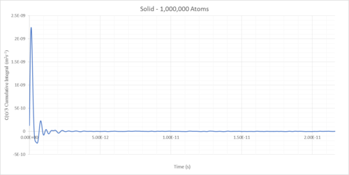
Minima and maxima in a VACF graph describe moments when the total force acting on a particle equals zero; essentially, points at which the atom is in a low-energy state (Figure 20). These represent areas where attractive and repulsive forces from surrounding atoms are equal. In the case of solids there are many well-ordered sites of zero force in which atoms move back and forth as a damped harmonic oscillator. This represents the vibration of an atom between those surrounding it (Figure 21). These occur regularly and so further demonstrate the greater level of order found within a solid than a liquid or gas. Liquids show very few minima and maxima, and quickly converge to zero velocity as random collisions occur.

Figure 21: Animation depicting vibrations of solid FCC lattice.

The harmonic oscillator VACF is the most regular and shows no decay. This is because it is a theoretical construct including no friction or collisions; its wavelength remains constant at approximately 40 timesteps as it oscillates backwards and forwards in a totally predictable fashion.

Figure 22: VACF integrated with time for a simulated gas.	Figure 23: VACF integrated with time for a large-scale simulated gas.
Figure 24: VACF integrated with time for a simulated liquid.	Figure 25: VACF integrated with time for a large-scale simulated liquid.
Figure 26: VACF integrated with time for a simulated solid.	Figure 27: VACF integrated with time for a large-scale simulated solid.

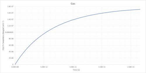
As more collisions occur, the velocity of each atom becomes more random (in the sense of uniform distribution between all directions), and therefore the VACF for each system converges to zero (Figures 22-27).

The diffusion coefficients of solids, liquids and gases can be determined as the integral of the VACF following convergence (Table 1).

The relatively large deviation between liquid diffusion coefficients acquired this way and using the MSD method is due to the concept of the long-time tail.² In a liquid model using hard-sphere interactions, a moving sphere will compress the liquid in front of it, and rarefy that behind. This causes a vortex flow around the sphere, pushing it forwards and resulting in velocity decay that is much slower than exponential. This long-time tail therefore always results in a greater value of D calculated from VACF data than MSD, as shown in Table 2. This is only prevalent in the liquid system, as gases do not have a high enough density to interact in this way, and solids do not diffuse.

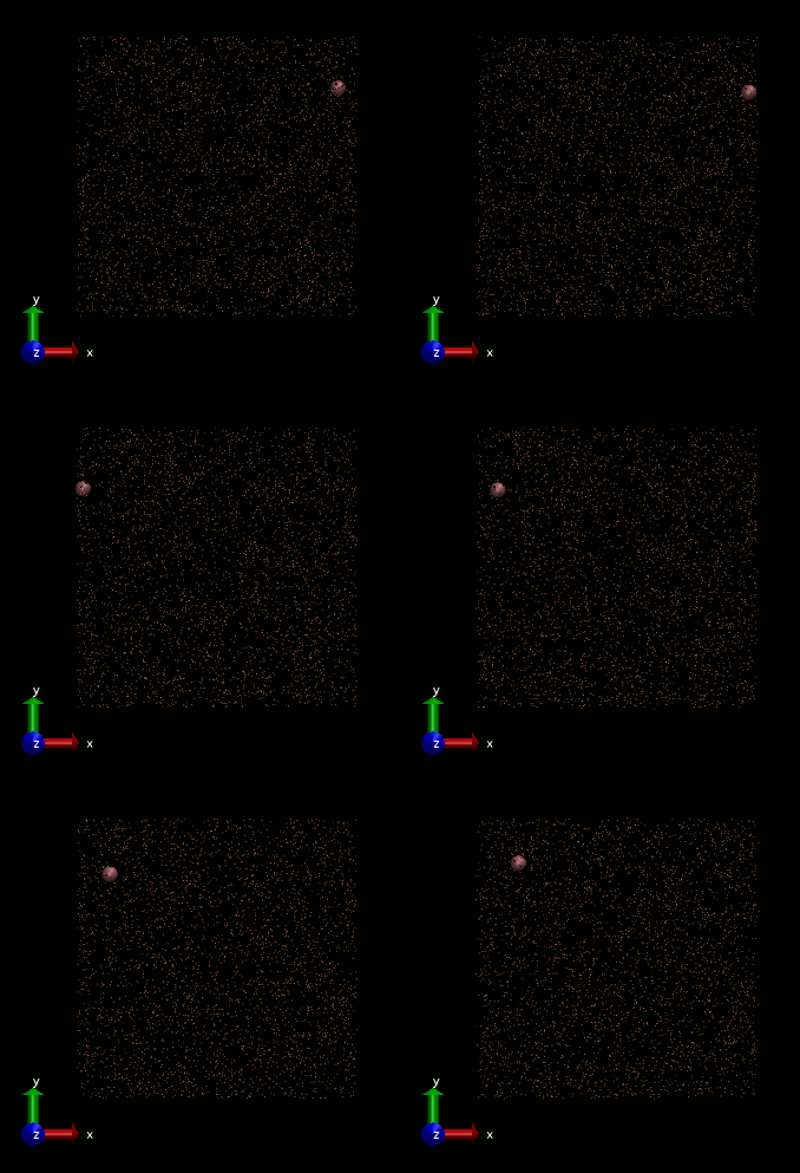
The simulations of gaseous systems were run again for a greater duration to ensure convergence (Figures 28 and 29).

JC: Excellent explanation of the VACF results.

Figure 28: MSD variation with time for a simulated gas for an extended period of time.

Figure 29: VACF integrated with time for a simulated gas for an extended period of time.

Diffusion Coefficient Results

Table 2: Diffusion coefficients for different phases; note all simulations used temperatures of 1.2 reduced units (143 K)

Phase	Density /reduced units	Density /1027 m-3	Diffusion Coefficient (MSD Method) /10-5 cm2s-1	Diffusion Coefficient (VACF Method) /10-5 cm2s-1
Gas	0.05	1.27	186	180
Liquid	0.8	20.35	4.64	4.81
Solid	1.2	30.53	~0	~0

The gas diffusion coefficient is of a similar order of magnitude as that found in literature.³ At the temperature used in this simulation, the literature value of the diffusion coefficient would be approximately 4600*10^-9 m²/s, whereas that found in this simulation is about 170. This is because the literature values correspond to a pressure of 1.013 bar (101 kPa) and that used in these simulations was approximately 21 bar (2.1 MPa). Diffusion coefficient varies inversely with pressure, so a D value of 4600*10^-9 m²/s at 21 bar corresponds to a D value of approximately 220*10^-9 m²/s at 1 bar, showing reasonable similarity to that found in these simulations.

The liquid diffusion coefficient is of the same order of magnitude as that found in literature (2.83*10^-5 cm²s^-1).⁴ Liquids are still susceptible to change of diffusion coefficient with temperature in accordance with the Stokes-Einstein equation.⁵ The temperature associated with the literature value is 90 K, compared to the simulated value of 144 K. Were the pressures identical in both cases, the value of D predicted using the Einstein-Stokes equation would be $\frac{144}{90}\times 2.83\times 10^{-5}{\mathrm{c}\mathrm{m}}^2{\mathrm{s}}^{-1}=4.53\times 10^{-5}{\mathrm{c}\mathrm{m}}^2{\mathrm{s}}^{-1}$. This shows good agreement with the values of 4.64 and 4.81 *10^-5 cm²s^-1 predicted by the MSD and VACF methods, respectively.

The solid diffusion coefficient is essentially zero due to the highly restricted freedom placed upon atoms in a high density face-centred cubic close-pack lattice.

JC: Great explanation and use of additional research and comparison with literature values. It would be good to explain briefly what system the literature results come from and how similar it is to your simulations.

References

(1) E. W. Lemmon, M. O. McLinden and D. G. Friend, in NIST Chemistry WebBook, NIST Standard Reference Database Number 69, National Institute of Standards and Technology, 1998.

(2) M. P. Allen and D. J. Tildesley, Computer simulation of liquids, Clarendon Press, 1989.

(3) S. Hi Lee, D. Kue Park and D. Bok Kang, Bull. Korean Chem. Soc. Song Hi Lee al, 2003, 24.

(4) J. Kestin, K. Knierim, E. A. Mason, B. Najafi, S. T. Ro and M. Waldman, J. Phys. Chem. Ref. Data, 1984, 13, 229–303.

(5) C. Cruickshank Miller, Math. Phys. Character, 1924, 106, 724–749.