Talk:Mod:AS12713Liquid

JC: General comments: All task completed and results well presented. Try to make your explanations clearer, more concise and more focused to demonstrate your understanding of the background material.

Introduction

The aim of this liquid simulations computational experiment is to investigate the computational simulation of chemical systems. Computer simulations are widely used to study a wide array of chemical phenomena, for example protein folding and the properties of biological systems such as lipid membranes. In this experiment molecular dynamics simulation will be used, which is one of the most powerful methods for the simulation of chemical systems. Molecular dynamics is method used for studying the physical movements of atoms and molecules, and is thus a type of N-body simulation.

The simulations of a simple liquid will be run on the High Performance Computing (HPC) system with a software package called Large-scale Atomic/Molecular Massively Parallel Simulator (LAMMPS). In order to visualise the data produced from the simulations a program called Visual Molecular Dynamics (VMD) was used to animate and analyse the trajectory of a molecular dynamics simulation.

Therefore, in order to simulate a liquid and investigate its properties, various ensembles, timesteps and algorithms were used. Additionally, the equilibration of the system, the heat capacity, the radial distribution function (RDF) and the diffusion enabled the structural properties of a simple liquid to be investigated when compared to a solid or a gas.

Introduction to Molecular Dynamics Simulation

Velocity-Verlet Algorithm

The velocity-Verlet algorithm is a numerical method used to solve Newton's equations of motion and is frequently used calculate the trajectories of particles in molecular dynamics simulations. This algorithm can be derived by assuming that the acceleration of an atom depends only on its position and not its velocity. In order to use this algorithm it is necessary to know the starting positions of the atoms(${\mathbf{x}}_i\left(0\right)$) and their velocities at the same time (${\mathbf{v}}_i\left(0\right)$). In this case, the velocity-Verlet algorithm is used to model the behaviour of a classic harmonic oscillator.

Figure 1. Graph showing the particle position as a function of time for analytical and velocity-Verlet algorithm using a timestep of 0.1s

Figure 2. Graph showing the energy as a function of time for the velocity-Verlet algorithm using a timestep of 0.1s

Figure 3. Graph showing the error as a function of time between analytical and velocity-Verlet algorithm using a timestep of 0.1s

Figure 4. Graph showing the fitted maximum error as a function of time between analytical and velocity-Verlet algorithm using a timestep of 0.1s

The analytical contains the value of the classical solution for the position at time t and is given by equation (1) below. Figure 1 shows the comparison of the classical solution and the solution given by the velocity-Verlet algorithm for the positions as a function of time. The graph shows that the position of an atom on a harmonic oscillator follows a cosine curve with a maximum value of +1.00 and a minimum value of -1.00. Additionally, the graphs shows that both solutions are appropriate for the harmonic oscillator because it behaves classically.

$$\begin{gathered} x\left(t\right)=A\cos (\omega t+\varphi ) \\ (1) \end{gathered}$$ where $x\left(t\right)$ is the position at time t, A = 1.00, $\omega$ = 1.00 and $\varphi$ = 0.00

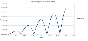
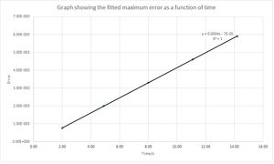
However, there is an error associated between the methods but it is not significant as can be seen from figure 1. The error contains the absolute difference between the analytical and the velocity-Verlet solution and is given by equation (2) below. Figure 3 shows the error calculated between the two methods and it can be seen that the error increases with time. The reason for this is that the error is additive since the Taylor expansion is being used in the velocity-Verlet algorithm. Figure 4 shows the maximum error as a function of time and from this it can be seen that as the simulation proceeds to longer times, the error between the classical and velocity-Verlet solutions increases linearly.

Error = $abs[x(t)-analytical]$ (2)

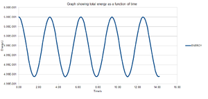
The energy contains the total energy of the oscillator for the velocity-Verlet solution and is given by equation (3) below. This is the sum of the kinetic and potential energies. Figure 2 shows the total energy as a function of time and it can be seen that there are periodic changes in the total energy. For a closed system, such as a simple harmonic oscillator, the total energy is expected to remain constant. Therefore, if the system progressively loses energy then this would suggest that the calculations being performed have some sort of error associated with them. However, since the velocity-Verlet algorithm is an approximation it would not be expected that the analytical and velocity-Verlet energies matched exactly.

$$\begin{gathered} E=\frac{1}{2}m{v}^2+\frac{1}{2}k{x}^2 \\ (3) \end{gathered}$$ where $m$ = 1.00, $k$ = 1.00, V(0) = 0.00 and X(0) = 1.00

For all the data and graphs shown above, a timestep of 0.1s was used for the simulation. The value of the timestep can be changed accordingly in order to ensure that the total energy does not change by more than 1% over the course of the simulation. In order to ensure this, a timestep value of below 0.2s has to be used because a timestep of 0.2s produces an error of 1% in the total energy between the analytical and velocity-Verlet algorithm. It is important to monitor the total energy of a physical system when modelling its behaviour numerically in order to ensure that the simulation is valid, has physical meaning and that there are no discrepancies from the analytical.

JC: Good choice of timestep and explanations.

Atomic Forces

Since the equations from quantum physics cannot be solved reasonably to determine the forces acting on a given configuration of atoms it is necessary to make approximations. From classical physics it is known that the force acting on an object is determined by the potential that it experiences. The force that a single atom feels is determined by the position of every other atom in the simulation. For many simple liquids, the interactions between each pair of atoms can be modelled extremely well using the Lennard-Jones potential, the equation of which for a single interaction is shown below by equation (4).

$$\begin{gathered} \varphi \left(r\right)=4ϵ(\frac{{\sigma }^{12}}{r^{12}}-\frac{{\sigma }^6}{r^6}) \\ (4) \end{gathered}$$ where $\varphi$ = potential energy, $ϵ$ = well-depth, r = separation between atoms and $\sigma$ = interatomic distance at which the potential reaches zero

The separation, $r_0$, at which the potential energy is zero:

$$\begin{gathered} \varphi \left(r_0\right)=4ϵ(\frac{{\sigma }^{12}}{(r_0{)}^{12}}-\frac{{\sigma }^6}{(r_0{)}^6}) \\ =0 \end{gathered}$$

$\frac{{\sigma }^{12}}{(r_0{)}^{12}}-\frac{{\sigma }^6}{(r_0{)}^6}=0$

${\sigma }^{12}(r_0{)}^6={\sigma }^6(r_0{)}^{12}$

$\sigma =r_0$

The force at this separation:

$F(r_0)=-\frac{d\varphi (r_0)}{d{r}_0}=-4ϵ(\frac{-12{\sigma }^{12}}{(r_0{)}^{13}}+\frac{6{\sigma }^6}{(r_0{)}^7})=-4ϵ(\frac{-12(r_0{)}^{12}}{(r_0{)}^{13}}+\frac{6(r_0{)}^6}{(r_0{)}^7})=-4ϵ(\frac{-12}{(r_0)}+\frac{6}{(r_0)})=\frac{24ϵ}{r_0}$

The equilibrium separation, $r_{eq}$:

$F(r)=-\frac{d\varphi (r)}{dr}=-4ϵ(\frac{-12{\sigma }^{12}}{r^{13}}+\frac{6{\sigma }^6}{r^7})=0$

$(\frac{-12{\sigma }^{12}}{r^{13}}+\frac{6{\sigma }^6}{r^7})=0$

$\frac{12{\sigma }^{12}}{r^{13}}=\frac{6{\sigma }^6}{r^7}$

$r_{eq}=\sqrt[6]{2}\sigma$

The well depth, $\varphi (r_{eq})$:

$\varphi (r_{eq})=4ϵ\frac{{\sigma }^{12}}{(2^{\frac{1}{6}}\sigma {)}^{12}}-4ϵ\frac{{\sigma }^6}{(2^{\frac{1}{6}}\sigma {)}^6}=4ϵ\frac{{\sigma }^{12}}{4{\sigma }^{12}}-4ϵ\frac{{\sigma }^6}{2{\sigma }^6}=ϵ-2ϵ=-ϵ$

Evaluating the integral $\underset{y}{\overset{x}{\int }}\varphi \left(r\right)\mathrm{d}r$ when $\sigma =ϵ=1.0$ using $x=\mathrm{\infty }$ and $y=2\sigma$, $2.5\sigma$, and $3\sigma$:

$\underset{y}{\overset{x}{\int }}\varphi \left(r\right)\mathrm{d}r=\underset{y}{\overset{x}{\int }}4ϵ(\frac{{\sigma }^{12}}{r^{12}}-\frac{{\sigma }^6}{r^6})\mathrm{d}r=4[\frac{-1}{11r^{11}}+\frac{1}{5r^5}{]}_y^x$

$\underset{2\sigma }{\overset{\mathrm{\infty }}{\int }}\varphi \left(r\right)\mathrm{d}r=4[\frac{-1}{11r^{11}}+\frac{1}{5r^5}{]}_{2\sigma }^{\mathrm{\infty }}=0-4(\frac{-1}{11(2^{11})}+\frac{1}{5(2^5)})=-0.0248$

$\underset{2.5\sigma }{\overset{\mathrm{\infty }}{\int }}\varphi \left(r\right)\mathrm{d}r=4[\frac{-1}{11r^{11}}+\frac{1}{5r^5}{]}_{2.5\sigma }^{\mathrm{\infty }}=0-4(\frac{-1}{11(2.5^{11})}+\frac{1}{5(2.5^5)})=-0.00818$

$\underset{3\sigma }{\overset{\mathrm{\infty }}{\int }}\varphi \left(r\right)\mathrm{d}r=4[\frac{-1}{11r^{11}}+\frac{1}{5r^5}{]}_{3\sigma }^{\mathrm{\infty }}=0-4(\frac{-1}{11(3^{11})}+\frac{1}{5(3^5)})=-0.00329$

Periodic Boundary Conditions

The realistic volumes of liquid cannot be simulated and in these simulations N will be between 1000 and 10000.

Estimating the number of water molecules in 1ml of water under standard conditions:

$\rho =\frac{m}{V}$

$m=\rho V=(1gm{l}^{-1})(1ml)=1g$

$moles=\frac{mass}{M_r}=\frac{1g}{18.02gmo{l}^{-1}}=0.0555mol$

Number of molecules = $(moles)(N_A)$ = (0.0555 mol) (6.022 x 10²³) = 3.34 x 10²²

Estimating the volume of 10000 water molecules under standard conditions:

$moles=\frac{N}{N_A}=\frac{10000}{N_A}$ = 1.66 x 10^-20 mol

mass = (1.66 x 10^-20) x (18.02) = 2.99 x 10^-19 g

$V=\frac{m}{\rho }$ = 2.99 x 10^-19 ml

Consider an atom at position (0.5, 0.5, 0.5) in a cubic simulation box which runs from (0, 0, 0) to (1, 1, 1). In a single timestep, it moves along the vector (0.7, 0.6, 0.2). At what point does it end up, after the periodic conditions have been applied?

The final position is (0.2, 0.1, 0.7)

Reduced Units

When using Lennard-Jones interactions it is typical to work in reduced units. In other words, all quantities in the simulation are divided by scaling factors. The result of this is that the values become more manageable. The reduced quantities are denoted by a star, and they take the following conversion factors:

Distance $r^{*}=\frac{r}{\sigma }$

Energy $E^{*}=\frac{E}{ϵ}$

Temperature $T^{*}=\frac{k_{B}T}{ϵ}$

The Lennard-Jones parameters for argon are $$\begin{gathered} \sigma =0.34\mathrm{n}\mathrm{m},ϵ \\ / \\ {k}_B=120\mathrm{K} \end{gathered}$$. If the Lennard-Jones cutoff is $r^{*}=3.2$, its real units is given by:

r = 3.2 x 0.34 nm = 1.09 nm

The well depth is given by:

$E=\frac{120k_B{N}_A}{1000}=-0.997kJmo{l}^{-1}$ (Negative since the well-depth = -$ϵ$)

The reduced temperature $T^{*}=1.5$ in real units is given by:

T = 1.5 x 120 = 180K

JC: All maths and calculations correct and nicely laid out.

Equilibration

Creating the Simulation Box

Before a simulation can be started it is necessary to know the initial states of all atoms in the system. The exact information required for each atom depends on the method of numerical integration used, but at the very least the starting position of each atom needs to be specified. However, generating the coordinates for atoms in a liquid is difficult since there is no long range order and so a single point of reference cannot be used to work out the positions of every other atom like in a solid. Therefore, instead of this a random position for each atom can be generated to produce atomic coordinates. However, this would create a disordered structure and cause larger problems when trying to run the simulation.

Giving atoms random starting coordinates causes problems in simulations because if the two atoms generated happen to be close together there would be significant repulsion and a high potential energy associated with this. This in turn would result in errors within the simulation process and hence it would be difficult to produce valid results.

JC: If a simulation is run from a starting configuration with very high repulsive forces the simulation is likely to be unstable and to require a much smaller timestep to prevent it from crashing.

Therefore, instead of this the atoms will be placed on the lattice points of a simple cubic lattice. This, of course, is not a situation in which the system is likely to be found physically. However, it turns out that if the simulation is run for enough time the atoms rearrange themselves into more realistic configurations.

The input file contains the line as shown below:

lattice sc 0.8

This command creates a grid of points forming a simple cubic lattice (one lattice point per unit cell). The parameter 0.8 specifies the number density (number of lattice points per unit volume). In the output file, the line below is seen:

Lattice spacing in x,y,z = 1.07722 1.07722 1.07722

This line indicates that the distance between the points of this lattice is 1.07722.

Proving that the lattice spacing corresponds to a number density of lattice points of 0.8:

Number density = The number of lattice points per unit volume

$V=1.07722^3=1.249$

$\frac{1}{1.249}=0.8$ (Since the unit cell only contains 1 lattice point)

For a face-centred cubic lattice with a lattice point number density of 1.2, the side length of the cubic unit cell is given by:

$V=\frac{4}{1.2}=3.33$ (The face-centred cubic lattice consists of 4 lattice points)

Length = $\sqrt[3]{V}=\sqrt[3]{3.33}=1.49$

For the face-centred cubic lattice, the number of atoms that would be created by the create_atoms command would be 4000. This value was obtained by considering the fact that the box contains 1000 unit cells of the lattice and there are 4 lattice points. Therefore, there should be 4000 atoms (1000 x 4).

JC: Correct.

Setting the Properties of the Atoms

The following commands are observed in the input script:

mass 1 1.0
pair_style lj/cut 3.0
pair_coeff * * 1.0 1.0

The first line above sets the mass for all type 1 atoms to mass 1.0.

The second line above specifies the cutoff point of pairwise interactions for the Lennard-Jones potential which in this case is specified at 3.0. This is the distance at which no significant interaction occurs.

JC: At the cutoff the potential is set to 0. Why is this used?

The third line above specifies the pairwise force field coefficients for all atoms. In this case the coefficients for all atoms are set to 1.0. The Lennard-Jones potential requires two force field coefficients $\sigma$ and $ϵ$, both of which have been set to 1.0.

Since X_i (0) and V_i (0) are specified, the velocity-Verlet algorithm will be used as described previously.

Running the Simulation

### SPECIFY TIMESTEP ###
variable timestep equal 0.001
variable n_steps equal floor(100/${timestep})
variable n_steps equal floor(100/0.001)
timestep ${timestep}
timestep 0.001

### RUN SIMULATION ###
run ${n_steps}
run 100000

The code used for the simulation is shown above. The purpose of these lines is to allow a variable to be defined once, such that all other values dependent on this variable will change accordingly. Additionally, the code enables the variable to be reused such that if a new set of conditions are required only the value of the variable at the beginning of the code has to be changed as oppose to changing all the values. Therefore, this code allows a specific timestep to be included in every simulation. If the simpler version of this code was used then the timestep values would have to be inputted manually in order to ensure that the simulation is running at a constant rate because the timestep has not been defined as a variable. Furthermore, in the simpler version of the code the number of steps was not determined by division and the duration of the computation not stated explicitly.

Checking Equilibration

Figure 5. Graph showing the reduced energy as a function of time using a timestep of 0.001s

Figure 6. Graph showing the reduced temperature as a function of time using a timestep of 0.001s

Figure 7. Graph showing the pressure as a function of time using a timestep of 0.001s

Figure 8. Graph showing the reduced energy as a function of time using various timesteps

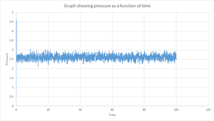
Plots of the reduced energy, reduced temperature and pressure against time for the 0.001s timestep can be seen in figures 5, 6 and 7. The simulation reaches equilibrium since each of the values for the reduced energy, reduced temperature and pressure level off and converge to an average value of -3.184, 1.250 and 2.580 respectively. Also, it can be seen from the graphs that there are constant fluctuations around these average values. By zooming in on each of the graphs it can be determined that this plateau begins at around 0.40s and thus this is the time it takes for the system to reach equilibrium.

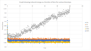
A plot of the reduced energy as a function of time using various timesteps is shown in figure 8. Choosing a particular timestep is a balancing act since the shorter the timestep the more accurately the results of the simulation will reflect the physical reality; short timesteps, however, mean that the same number of simulation steps cover a shorter amount of actual time, and this is very unhelpful if the process under investigation requires observation over a long time. Of the five timesteps used, the largest to give acceptable results is either 0.001s or 0.0025s. Both these timestep converged to essentially the same energy value with the smallest fluctuations and hence both would produce acceptable and accurate results. However, a timestep of 0.0025s is chosen over 0.001s because it requires less computational time and thus gives rise to a faster simulation. Contrastingly, the simulation with the timestep of 0.0015s is a particularly bad choice because it does not converge to a value and thus does not reach equilibrium. Also, there is a large variance between the values since the reduced energy increases with time. This in turn means that the timestep of 0.0015s would not be appropriate for any calculations.

JC: Good, thorough analysis. The energy should not depend on the timestep, so the timesteps of 0.0075 and 0.01 are not suitable.

Running Simulations Under Specific Conditions

Up until now all the simulations have been run such that the number of particles and the volume of the simulation cell are held constant. The energy is also constant within a certain degree of error, which is introduced by the approximations made to run the simulation. If the simulation is working properly, then the pressure and temperature of the system should also reach a constant average value, even though there will be fluctuations. Ensembles are used in statistical mechanics in order to represent different experimental conditions. The simulations carried out so far are described by the microcanonical, or NVE, ensemble. The following simulations will be run under NpT conditions (isobaric-isothermal ensembles).

Thermostats and Barostats

The equipartition theorem states that, on average, every degree of freedom in a system at equilibrium will have $\frac{1}{2}{k}_{B}T$ of energy. In this system with N atoms, each with three degrees of freedom (translational, vibrational and rotational), the following can be written:

$E_K=\frac{3}{2}N{k}_{B}T$

$\frac{1}{2}\sum _i{m}_i{v}_i^2=\frac{3}{2}N{k}_{B}T$

At the end of every timestep, the left hand side of the above equation can be used to calculate the kinetic energy, then divided by $\frac{3}{2}N{k}_B$ to get the instantaneous temperature $T$. In general, $T$ will fluctuate, and will be different to the target temperature, $\mathfrak{𝔗}$, which is a value specified in the input script. It is possible to change the temperature by multiplying every velocity by a constant factor, $\gamma$.

If $T>\mathfrak{𝔗}$, then the kinetic energy of the system is too high, and needs to be reduced. ($\gamma <1$)

If $T<\mathfrak{𝔗}$, then the kinetic energy of the system is too low, and needs to be increased. ($\gamma >1$)

The constant factor, $\gamma$, needs to be chosen such that $T=\mathfrak{𝔗}$. Two equations, as shown below, can be written and solved to determine $\gamma$.

$\frac{1}{2}\sum _i{m}_i{v}_i^2=\frac{3}{2}N{k}_{B}T$

$\frac{1}{2}\sum _i{m}_i{\left(\gamma v_i\right)}^2=\frac{3}{2}N{k}_B\mathfrak{𝔗}$

Both the equations above were rearranged for $3N{k}_B$, then equated and solved as shown below:

$3N{k}_B=\frac{\sum _i{m}_i{v}_i^2}{T}$

$3N{k}_B=\frac{{\gamma }^2\sum _i{m}_i{v}_i^2}{\mathfrak{𝔗}}$

$\frac{{\gamma }^2\sum _i{m}_i{v}_i^2}{\mathfrak{𝔗}}=\frac{\sum _i{m}_i{v}_i^2}{T}$

$\gamma =\sqrt{\frac{\mathfrak{𝔗}}{T}}$

JC: Good derivation and understanding of how thermostats work.

Examining the Input Script

### MEASURE SYSTEM STATE ###
thermo_style custom step etotal temp press density
variable dens equal density
variable dens2 equal density*density
variable temp equal temp
variable temp2 equal temp*temp
variable press equal press
variable press2 equal press*press
fix aves all ave/time 100 1000 100000 v_dens v_temp v_press v_dens2 v_temp2 v_press2
run 100000

A section of the input script is shown above and instructs LAMMPS to bring the system to the required state. The first command, thermo_style, controls which thermodynamic properties are recorded. The next lines are used to measure average thermodynamic properties for the system. In order to draw the equations of state, the average temperature, pressure, density and the statistical errors in these quantities need to be known.

The three numbers 100, 1000 and 100000 are important for the simulation because they correspond to N_every, N_repeat and N_freq. The first number determines how frequently an input value should be utilised for the average. In this case, every 100th input is taken and used in subsequent calculations. The second number specifies the number of input values used for determining the averages. In this case, 1000 values contribute towards the average. The third number sets the number of timestep values that pass before the average is calculated. In this case, 100000 timesteps pass before an average is obtained.

Therefore, values will be taken every 0.1s with 1000 measurements contributing to the average and a time simulated of 100s.

Plotting the Equations of State

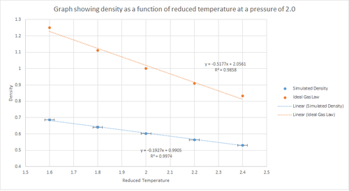
Five temperature were chosen above the critical temperature, $T^{*}=1.5$, and two pressures. In this case, the reduced temperatures chosen were 1.6, 1.8, 2.0, 2.2 and 2.4. All temperatures have to be above the critical temperature because this is a requirement for the substance to behave as a fluid. These were all run at two different pressures of 2.0 and 3.0. These specific values for the pressure were selected because from figure 7 it can be seen that the equilibrium value for the pressure is approximately 2.5. Hence, the two pressure values chosen are close to this equilibrium value. This gives ten phase points; five temperatures at each pressure. A timestep value of 0.0025s was used as this previously produced accurate results.

The density predicted by the Ideal Gas Law:

$PV=N{k}_{B}T$

$\frac{N}{V}=\frac{p}{k_{B}T}$

$\frac{N}{V}=\frac{p}{T}$ (since in reduced units $k_B=1$)

Figure 9. Graph showing the density as a function of reduced temperature at a pressure of 2.0

Figure 10. Graph showing the density as a function of reduced temperature at a pressure of 3.0

The plots shown in figures 9 and 10 above shows how the density changes with temperature and pressure. The graphs show that as the temperature increases the density decreases linearly. Also, there is a line corresponding to the density predicted by the Ideal Gas Law at both pressures. From this it can be seen that the simulated density is lower than that predicted by the Ideal Gas Law. This can be rationalised by considering the assumptions of the ideal gas model. The ideal gas model states that the density is proportional to the temperature at constant pressure. This model assumes that all atoms can be treated as point charges that do not interact. However, in the simulations performed this is not the case since the atoms interact via interatomic potential, such as the Lennard-Jones potential. Therefore, this means that the density at any given point, under the ideal gas model, will be higher than the simulated density. The discrepancy between the Ideal Gas Law and the simulation increases with an increase in pressure. This is because, at constant temperature, the density is proportional to the pressure.

JC: Why do you plot a line of best fit for the ideal gas data, you know the exact equation of state for an ideal gas, N/V = p/kT. The atoms in the ideal gas are not point charges, they are non-interacting. How does the discrepancy between the ideal gas and simulation results change with temperature?

Calculating Heat Capacities Using Statistical Physics

In statistical thermodynamics many quantities can be calculated by considering how far the system is able to fluctuate from its average equilibrium state. For example, if the temperature is held constant, then the total energy must be fluctuating. The magnitude of these fluctuations gives information about the heat capacity of the system, in accordance with the equation shown below.

$C_V=\frac{\partial E}{\partial T}=\frac{\mathrm{V}\mathrm{a}\mathrm{r}\left[E\right]}{k_B{T}^2}=N^2\frac{⟨E^2⟩-{⟨E⟩}^2}{k_B{T}^2}$

The simulations were run at ten phase points; two densities at 0.2 and 0.8 will run at the temperature values of 2.0, 2.2, 2.4, 2.6 and 2.8. An example of one of the input scripts used to run the simulation is shown below.

### DEFINE SIMULATION BOX GEOMETRY ###
lattice sc 0.2 ### The density was varied here (0.2 and 0.8)
region box block 0 15 0 15 0 15
create_box 1 box
create_atoms 1 box

### DEFINE PHYSICAL PROPERTIES OF ATOMS ###
mass 1 1.0
pair_style lj/cut/opt 3.0
pair_coeff 1 1 1.0 1.0
neighbor 2.0 bin

### SPECIFY THE REQUIRED THERMODYNAMIC STATE ###
variable T equal 2.0 ### The temperature was varied here (2.0, 2.2, 2.4, 2.6, 2.8)
variable timestep equal 0.0025 ### This timestep was found to be the most appropriate

### ASSIGN ATOMIC VELOCITIES ###
velocity all create ${T} 12345 dist gaussian rot yes mom yes

### SPECIFY ENSEMBLE ###
timestep ${timestep}
fix nve all nve 

### THERMODYNAMIC OUTPUT CONTROL ###
thermo_style custom time etotal temp press
thermo 10

### RECORD TRAJECTORY ###
dump traj all custom 1000 output-1 id x y z

### SPECIFY TIMESTEP ###

### RUN SIMULATION TO MELT CRYSTAL ###
run 10000
unfix nve
reset_timestep 0

### BRING SYSTEM TO REQUIRED STATE ###
variable tdamp equal ${timestep}*100
fix nvt all nvt temp ${T} ${T} ${tdamp} ### Changed as per the script
run 10000
reset_timestep 0
unfix nvt ### Switching off the thermostat 
fix nve all nve 

### MEASURE SYSTEM STATE ###
thermo_style custom step etotal temp atoms vol
variable etotal equal etotal
variable etotal2 equal etotal*etotal
variable temp equal temp
variable temp2 equal temp*temp
variable X equal atoms
variable X2 equal atoms*atoms
variable vol equal vol
fix aves all ave/time 100 1000 100000 v_etotal v_etotal2 v_temp v_temp2  
run 100000

variable aveetotal equal f_aves[1]
variable aveetotal2 equal f_aves[2]
variable avetemp equal f_aves[3]
variable ave2etotal equal f_aves[1]*f_aves[1]
variable heatcapacity equal ${X2}*(${aveetotal2}-${ave2etotal})/(${avetemp}*${avetemp}) ### Equation for calculating the heat capacity
variable heatcapacityvolume equal (${X2}*(${aveetotal2}-${ave2etotal})/(${avetemp}*${avetemp}))/vol ### Equation for calculating the heat capacity per unit volume    

print "Averages"
print "--------"
print "Temperature: ${avetemp}"
print "Heat Capacity: ${heatcapacity}"
print "Heat Capacity Volume: ${heatcapacityvolume}"

Figure 11. Graph showing the heat capacity over volume as a function of reduced temperature at a density of 0.2 and 0.8

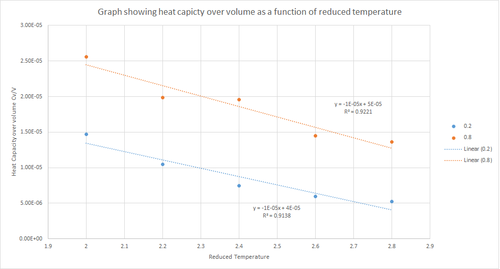The output results from the input code above were used to plot heat capacity over volume as a function of reduced temperature for the densities 0.2 and 0.8; the results of which are shown in figure 11 above. This graph shows that, in general, Cv/V decreases with increasing temperature for both density values. Heat capacity is defined as the energy required by a substance to raise the temperature of the system by one kelvin. The general trend does not follow the expected one; the heat capacity should increase with an increase in temperature. The fact that figure 11 shows that heat capacity decreases with increasing temperature can be explained by considering that the energy levels become closer together at higher temperatures. Thus, at a higher temperature less energy would be required in order to populate energy levels than at a lower temperature. In other words, less energy is required for excitation to higher energy levels. Furthermore, figure 11 shows that the heat capacity when the density is 0.2 is lower than when the density is 0.8. This is because at a higher density there are a greater number of particles per unit volume and so a larger amount of energy is required to raise the temperature of the system by one kelvin because there are more particles to absorb the energy.

JC: Good explanation.

Structural Properties and the Radial Distribution Function

The structure of systems that are simulated can be characterised by using Radial Distribution Functions (RDF), which are denoted by $g(r)$. Calculating the RDF for a simulation is very useful since it gives an indication of the distances from an atom at which its nearest neighbours can be found. Also, it is a quantity that can be accessed experimentally, and so provides a good check that the force field in the simulation is correctly reproducing the structural features. VMD will be used to calculate the RDF for the solid, liquid and vapour phases of the Lennard-Jones fluid. The values for the density and temperature to be used for the simulations were determined by analysing the phase diagram for the Lennard-Jones system. The values for each phase are summarised below:

Solid: Temperature = 1.2, Density = 1.2

Liquid: Temperature = 1.2, Density = 0.8

Vapour: Temperature = 1.2, Density = 0.05

Figure 12. Graph showing g(r) as a function of distance for the solid, liquid and vapour phases

Figure 13. Graph showing the integral of g(r) as a function of distance for the solid, liquid and vapour phases

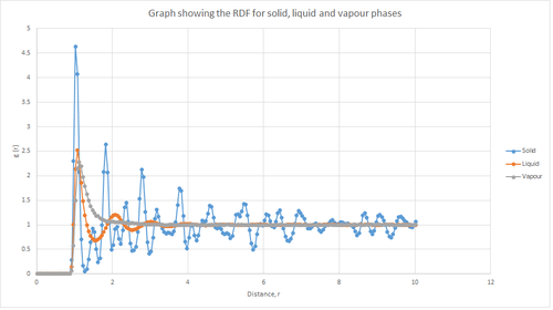
The plot shown in figure 12 above shows the differences between the RDFs of solid, liquid and vapour phases. The RDF is used to provide information about the structure of the system by describing the variation in the probability of finding particles. As can be seen from figure 12, the RDF of the vapour phase indicates that there is a high probability of finding the first neighbour, as indicated by the single peak. However, this probability decreases rapidly as the distance r increases, which in turn confirms that the molecules in a gas are far apart and randomly dispersion; hence the probability of finding another atom is relatively low. Also, this single peak is relatively broad which further emphasises that a gas is a highly disordered system.

From figure 12, the RDF of the liquid phase displays multiple peaks, of which three are well-defined. This arises from the fact that a liquid has some degree or order and hence liquids have a more structured environment, such that they form solvation shells. Additionally, it can be seen that the 3 peaks decrease in height as the distance increases. The peak closest to the reference atom (i.e. the first peak of the RDF)for the liquid phase is larger than that for the vapour phase. This is because a liquid is denser than a gas.

The RDF of the solid phase, as shown in figure 12, has many well-defined peaks due to its rigid structure and hence the nearest neighbours are well-defined. The solid phase has the highest density and hence the peak closest to the reference atom is the largest. All the graphs eventually level off to a value of 1 and at this point the density of all the phases is approximately constant.

JC: The RDFs level off to 1 as this is the bulk density for that phase, however, the peaks in the solid RDF even at large distances indicate that the solid has long range order.

Figure 14. Face-centred cubic crystal structure showing the three nearest neighbours from the RDF of solid phase

Figure 15. Graph showing the integral of g(r) as a function of radial extension for the first three peaks for the solid phase

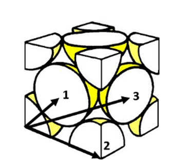
Figure 14 above illustrates the lattice sites the first three peaks correspond to from the RDF of the solid phase. The first three peaks give the distance of the three closest atoms to the reference. The first three maxima peaks from the solid phase RDF shown in Figure 12 are (1.025, 4.636), (1.475, 0.9221) and (1.825, 2.641). Therefore, using this it can be deduced that the lattice spacing is equal to the radial distance from the RDF origin to the second peak. Hence, the lattice spacing is equal to 1.475.

JC: Good diagram of an fcc lattice. Did you calculate the lattice parameter from the first or third peak as well?

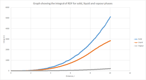
Figure 13 above shows the RDF integral as a function of radial extension for the solid, liquid and vapour phases. This shows that the solid phase has the largest area under $g(r)$, which reflects that the solid has the largest density. It can also be seen that the liquid phase has the next largest area, followed by the vapour phase which has the smallest area. The coordination number for each of the first three peaks in the solid phase can be determined from figure 15 above.

The coordination number corresponding to the first peak (first nearest neighbour) at a radial extension of 1.025 = 12 - 0 = 12

The coordination number corresponding to the second peak (second nearest neighbour) at a radial extension of 1.475 = 18 - 12 = 6

The coordination number corresponding to the third peak (third nearest neighbour) at a radial extension of 1.825 = 42 - 18 = 24

Dynamical Properties and the Diffusion Coefficient

Mean Squared Displacement

In statistical mechanics, the mean squared displacement (MSD), is a measure of the deviation over time between the position of a particle and a reference position. It is the most common measure of the spatial extent of random motion. From the phase diagram of the Lennard-Jones potential, it was found that a temperature of 1.2 and a density of 1.2 produced a solid phase; the liquid phase was produced by a temperature of 1.2 and density of 0.8; the vapour phase was produced by a temperature of 1.2 and density of 0.05.

Figure 16. Graph showing the MSD as a function of timestep for solid phase for small system

Figure 17. Graph showing the MSD as a function of timestep for liquid phase for small system

Figure 18. Graph showing the MSD as a function of timestep for vapour phase for small system

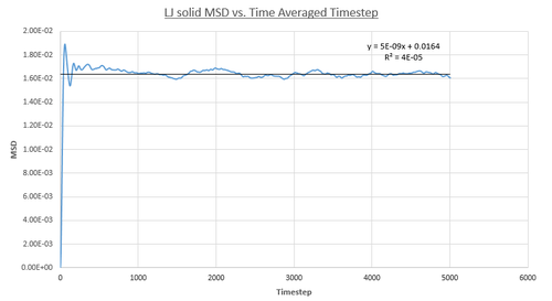
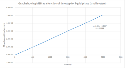
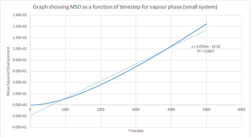
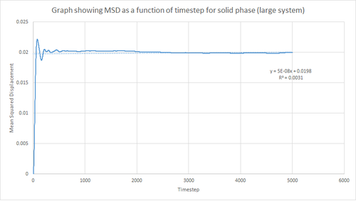
Figures 16, 17 and 18 above show the MSD as a function of timestep for the solid, liquid and vapour phases for 8,000 atoms. In the solid phase, the atoms are less able to be diffused due to the rigid lattice structure, whereas in the liquid and vapour phase the atoms are expected to move in accordance with Brownian motion since there are less restrictions in terms of fixed atomic positions. This in turn means that the MSD saturates rapidly to give a value which corresponds to atomic vibrations. As shown by figure 16, this results in a large initial increase in MSD for the solid phase followed by a subsequent plateau. Additionally, this graph shows an oscillatory-type of behaviour which in turn suggests that the displacement of the atoms are behaving like a damped harmonic oscillator.

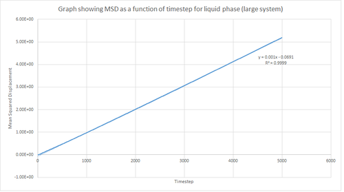
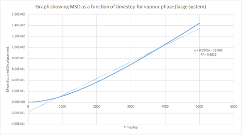
On the other hand, the liquid and vapour phase plots show that the MSD has a close linear dependence on time. The MSD for the liquid phase has complete linearity with an R² value of 0.9999, which in turn suggests that the trajectories of the atoms are completely randomised through frequent collisions. The MSD for the vapour phase is also linear, however, it is slightly curved at the beginning suggesting that atomic movements are not random at the start of the simulation but as time progresses the movements become randomised.

From the figures above it can also be seen that the vapour phase has a significantly larger MSD than the other phases. This is due to the fact that the atoms in the vapour phase have large translational velocities and weak interatomic interactions. Additionally, it can be seen that the liquid phase has a larger MSD than the solid phase because in the liquid phase there is no long range order that holds atoms in fixed positions. Therefore, this agrees with what was expected.

Finally, it can be seen that the gradient of the MSD graph for the vapour phase is much larger than that of the MSD for the liquid phase. This in turn agrees with the fact that gases are less ordered than liquids due to greater thermal motion in the vapour phase and hence Brownian motion becomes more pronounced. Also, in the vapour phase, until the atoms collide with each other the atom moves at constant velocity and thus the MSD is proportional to t² at the beginning of the simulation (curved region).

JC: You are right that initially the MSD is proportional to t^2, but this means that initially the motion is not diffusive. Therefore to calculate the diffusion coefficient you should only fit a straight line to the linear part of the MSD graph when the simulation has reached the diffusive regime.

This procedure was repeated for the MSD data given from the one million atom simulations. Figures 19, 20 and 21 below show the plots of these simulations. By comparing the simulations run for 8,000 atoms and 1 million atoms, it is evident that the graphs are essentially identical. Hence, the same observations and reasoning as outlined above apply for these graphs. Also, from this it can be concluded that 8,000 atoms is sufficient to perform these simulations and should be used instead of 1 million atoms since it is less expensive computationally.

Figure 19. Graph showing the MSD as a function of timestep for solid phase for large system

Figure 20. Graph showing the MSD as a function of timestep for liquid phase for large system

Figure 21. Graph showing the MSD as a function of timestep for vapour phase for large system

The equation shown below was used to calculate the diffusion coefficient of the atoms in each phase for 8,000 atoms and 1 million atoms. Therefore, using this, the diffusion coefficient was calculated by multiplying the gradient of the graph by 1/6 and dividing this value by the timestep value (0.002), in order to convert from the number of timesteps to the time in seconds. The diffusion coefficient values calculated are summarised in table 1 below.

$D=\frac{1}{6}\frac{\partial ⟨r^2\left(t\right)⟩}{\partial t}$

Table 1. The calculated diffusion coefficient values for the solid, liquid and vapour phases for 8000 and 1 million atoms

Phase	D / m2s-1 (8000 atoms)	D / m2s-1 (1 million atoms)
Solid	$4.17\times 10^{-7}$	$4.17\times 10^{-6}$
Liquid	$8.33\times 10^{-2}$	$8.33\times 10^{-2}$
Vapour	$2.53$	$2.54$

Table 1 above shows that the sample size does not have much of an effect in terms of the diffusion coefficient as the values are relatively similar. It can also be seen that the diffusion coefficient for the vapour phase is greater than that for the liquid phase which in turn is greater than that for the solid phase (D_Gas > D_Liq > D_Sol). This is the expected result because atoms in the vapour phase have large translational velocities and weak interatomic forces in comparison to the other phases. As well as this, the interatomic distance is much larger for the vapour phase in comparison to the liquid and solid phase. Thus, the more ordered the system, the lower the diffusion coefficient and the slower the rate of diffusion.

Velocity Autocorrelation Function

The diffusion coefficient can also be calculated using the velocity autocorrelation function (VACF), which is denoted by:

$C\left(\tau \right)=⟨\mathbf{v}\left(t\right)\cdot \mathbf{v}(t+\tau )⟩$

This function describes how different the velocity of an atom will be at time $t+\tau$ to its velocity at time $t$. At long times, it is expected that $C\left(\mathrm{\infty }\right)=0$, because the velocities of atoms should become uncorrelated at very long times. This in turn means that the velocity of an atom at a particular time should not depend on its velocity a long time in the past. The diffusion coefficient can be calculated by integrating the function shown below.

$D=\frac{1}{3}\underset{0}{\overset{\mathrm{\infty }}{\int }}\mathrm{d}\tau ⟨\mathbf{v}\left(0\right)\cdot \mathbf{v}\left(\tau \right)⟩$

The normalised VACF for a 1D harmonic oscillator is given by:

$C\left(\tau \right)=\frac{\underset{-\mathrm{\infty }}{\overset{\mathrm{\infty }}{\int }}v\left(t\right)v(t+\tau )\mathrm{d}t}{\underset{-\mathrm{\infty }}{\overset{\mathrm{\infty }}{\int }}{v}^2\left(t\right)\mathrm{d}t}$

The equation for the evolution of the position of a 1D harmonic oscillator as a function of time, as shown above, is used to evaluate the normalised VACF for a 1D harmonic oscillator as shown below.

The equation for a classic harmonic oscillator is given by:

$x(t)=Acos(\omega t+\varphi )$

The derivative of the position was taken with respect to time to give the velocity of the harmonic oscillator:

$v(t)=\frac{dx(t)}{dt}=-A\omega sin(\omega t+\varphi )$

This result can then be substituted into the integral for the normalised VACF for a 1D harmonic oscillator:

$C(\tau )=\frac{\underset{-\mathrm{\infty }}{\overset{\mathrm{\infty }}{\int }}[-A\omega sin(\omega t+\varphi )][-A\omega sin(\omega (t+\tau )+\varphi )]dt}{\underset{-\mathrm{\infty }}{\overset{\mathrm{\infty }}{\int }}[-A\omega sin(\omega t+\varphi ){]}^{2}dt}$

$C(\tau )=\frac{\underset{-\mathrm{\infty }}{\overset{\mathrm{\infty }}{\int }}[-A\omega sin(\omega t+\varphi )][-A\omega sin(\omega t+\omega \tau +\varphi )]dt}{\underset{-\mathrm{\infty }}{\overset{\mathrm{\infty }}{\int }}[-A\omega sin(\omega t+\varphi ){]}^{2}dt}$

The trigonometry identity, $sin(a+b)=sin(a)cos(b)+cos(a)sin(b)$, can be utilised. In this case, let $a=\omega t+\varphi$ and $b=\omega \tau$. Therefore, the above equation simplifies to:

$C(\tau )=\frac{\underset{-\mathrm{\infty }}{\overset{\mathrm{\infty }}{\int }}[-A\omega sin(a)][-A\omega sin(a+b)]dt}{\underset{-\mathrm{\infty }}{\overset{\mathrm{\infty }}{\int }}[-A\omega sin(a){]}^{2}dt}$

$C(\tau )=\frac{\underset{-\mathrm{\infty }}{\overset{\mathrm{\infty }}{\int }}[-A\omega sin(a)][-A\omega (sin(a)cos(b)+cos(a)sin(b))]dt}{\underset{-\mathrm{\infty }}{\overset{\mathrm{\infty }}{\int }}[-A\omega sin(a){]}^{2}dt}$

$C(\tau )=\frac{\underset{-\mathrm{\infty }}{\overset{\mathrm{\infty }}{\int }}[(-A\omega {)}^{2}si{n}^2(a)cos(b)][(-A\omega {)}^{2}sin(a)cos(a)sin(b))]dt}{\underset{-\mathrm{\infty }}{\overset{\mathrm{\infty }}{\int }}[-A\omega sin(a){]}^{2}dt}$

This equation can be simplified further by splitting the integral into two separate fractions. Also, since $A\omega$ and $b=\omega \tau$ are both constants, they can be taken outside the integral. This process is shown below:

$C(\tau )=\frac{(-A\omega {)}^{2}cos(b)\underset{-\mathrm{\infty }}{\overset{\mathrm{\infty }}{\int }}[si{n}^2(a)]}{(-A\omega {)}^2\underset{-\mathrm{\infty }}{\overset{\mathrm{\infty }}{\int }}[si{n}^2(a)]dt}+\frac{(-A\omega {)}^{2}sin(b)\underset{-\mathrm{\infty }}{\overset{\mathrm{\infty }}{\int }}[sin(a)cos(a)]}{(-A\omega {)}^2\underset{-\mathrm{\infty }}{\overset{\mathrm{\infty }}{\int }}[si{n}^2(a)]dt}$

$C(\tau )=cos(b)+\frac{sin(b)\underset{-\mathrm{\infty }}{\overset{\mathrm{\infty }}{\int }}[sin(a)cos(a)]}{\underset{-\mathrm{\infty }}{\overset{\mathrm{\infty }}{\int }}[si{n}^2(a)]dt}$

This can be further simplified owing to the fact that the integral of an odd function, between two limits equidistant from the origin (i.e. using symmetric limits), is equal to zero. Therefore, the above equation becomes:

$C(\tau )=cos(b)=cos(\omega \tau )$

JC: Good, clear derivation.

Figure 22. Graph showing VACF as a function of timestep for solid and liquid phase for small system, plotted with the analytical solution for 1D harmonic oscillator

Figure 23. Graph showing VACF as a function of timestep for solid and liquid phase for large system, plotted with the analytical solution for 1D harmonic oscillator

Figure 24. Graph showing VACF as a function of timestep for solid phase for small system

Figure 25. Graph showing VACF as a function of timestep for liquid phase for small system

Figure 26. Graph showing VACF as a function of timestep for vapour phase for small system

Figure 27. Graph showing VACF as a function of timestep for solid phase for large system

Figure 28. Graph showing VACF as a function of timestep for liquid phase for large system

Figure 29. Graph showing VACF as a function of timestep for vapour phase for large system

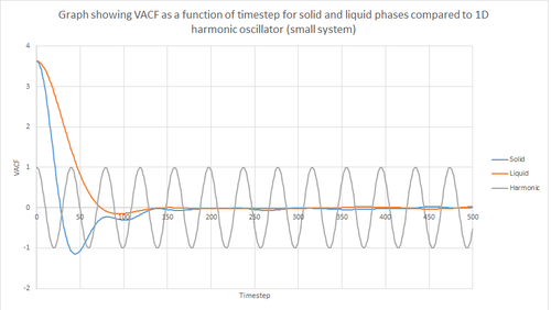
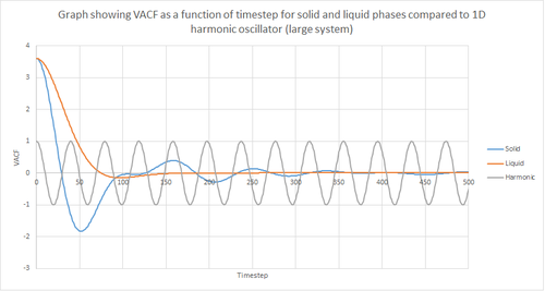
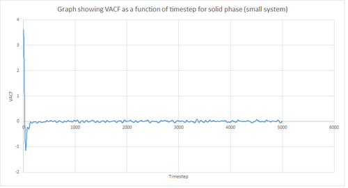
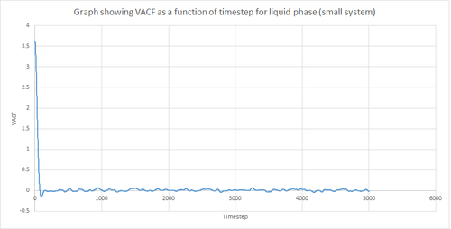
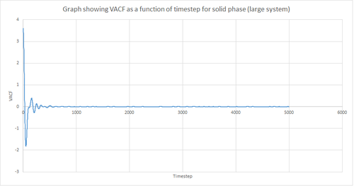
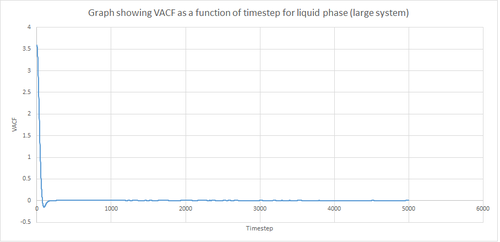
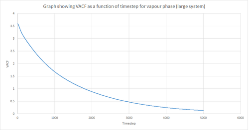
Figures 22 and 23 above show the VACF as a function of timestep for 8,000 and 1 million atoms respectively, for the solid and liquid phase, with the superimposed analytical solution for the 1D harmonic oscillator. It can be seen from the graphs that, for the liquid phase, there is a small minimum peak then the curve begins to plateau towards zero. On the other hand, the VACF for the solid phase shows a sharp decrease in velocity which then oscillates until it reaches zero. It can also be seen that the solid phase has one major minimum peak before it begins to oscillate, and form several smaller minima. The major minima for the solid a liquid phases represent the largest maximum velocity achieved by the oscillatory atom motions within each system.

A major feature of the 1D harmonic oscillator VACF is the oscillatory behaviour of the system. For a harmonic oscillator, by definition, the restoring force is constant. In the solid phase, the positions of the atoms are fixed (regularly ordered atoms in a closely packed structure) and hence harmonic oscillatory behaviour would be expected for this system. This can be seen in figure 27, whereby there is evident oscillatory behaviour as the atoms vibrate. However, these oscillations are unequal in magnitude and eventually decays off toward zero (damped harmonic oscillations). For the case of the liquid phase, the Lennard-Jones fluid experiences relatively strong interatomic forces and a relatively high density. However, as a result of Brownian motion (atoms do not have fixed positions in liquid), there is a higher rate of diffusion. Thus, this explains the plot shown in figure 28 in which the VACF is oscillatory as the start but then decays rapidly towards zero (much faster than for the solid phase). Therefore, the differences between the VACF plots for the solid and liquid phase arise from the difference in the order of the system, along with the structure.

The harmonic oscillator VACF is very different to the Lennard-Jones solid and liquid because the harmonic oscillator ignores forces that act against the oscillatory behaviour. For the Lennard-Jones plots, the potential tends towards zero at large displacements, hence the atoms exert smaller forces and become uncorrelated. Contrastingly, for the harmonic oscillator the atomic forces increase at large displacements. Hence, the atoms will be close to each other and have perfectly correlated velocities. This in turn explains the fact that the VACF for solid and liquid tend towards zero over the course of the simulation, while the harmonic oscillator does not. Also, a harmonic oscillator is isolated and thus never collides with other particle, thus the system continues oscillating.

JC: It is the collisions with other particles that leads to decorrelation of the particle velocities.

The diffusion coefficient is related to the VACF as shown by the equation below:

$D=\frac{1}{3}\underset{0}{\overset{\mathrm{\infty }}{\int }}\mathrm{d}\tau ⟨\mathbf{v}\left(0\right)\cdot \mathbf{v}\left(\tau \right)⟩$

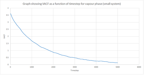
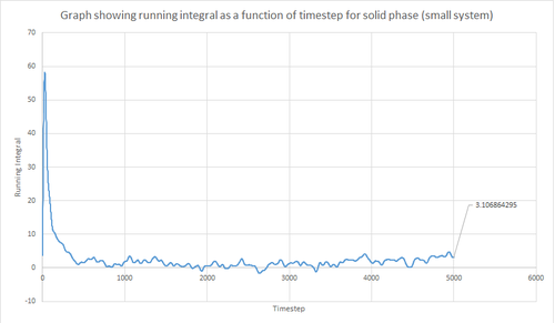
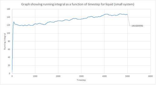
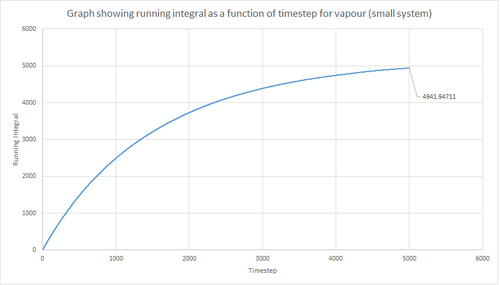
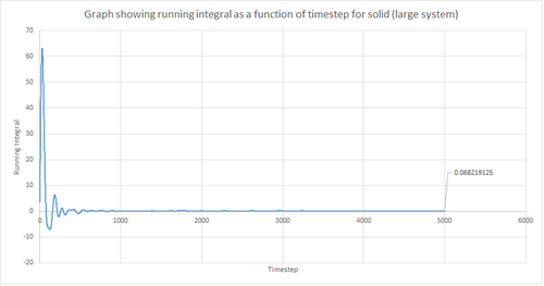
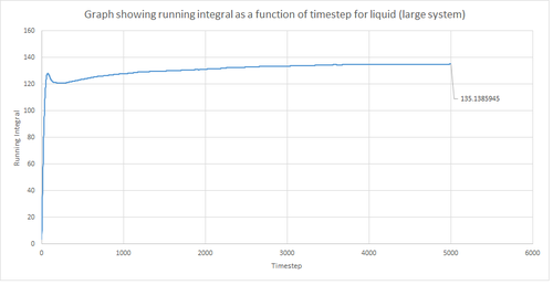
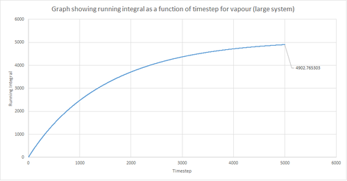
The trapezium rule, the general equation of which is shown below, was used to approximate the integral under the VACF for the solid, liquid and gas phase. The running integral was calculated by finding the area underneath the VACF curve between each timestep (Δt=1) and adding it to the total cumulative area from subsequent timesteps. Thus, from this the total integral can be determined from the last data point of the running integral plots, of which are shown in the figures below.

$\underset{a}{\overset{b}{\int }}f(x)dx\approx (b-a)\left[\frac{f(a)+f(b)}{2}\right]$

Figure 30. Graph showing running integral as a function of timestep for solid phase for small system

Figure 31. Graph showing running integral as a function of timestep for liquid phase for small system

Figure 32. Graph showing running integral as a function of timestep for vapour phase for small system

Figure 33. Graph showing running integral as a function of timestep for solid phase for large system

Figure 34. Graph showing running integral as a function of timestep for liquid phase for large system

Figure 35. Graph showing running integral as a function of timestep for vapour phase for large system

Table 2. The calculated diffusion coefficient values for the solid, liquid and vapour phases for 8000 and 1 million atoms using VACF

Phase	D / m2s-1 (8000 atoms)	D / m2s-1 (1 million atoms)
Solid	$2.07\times 10^{-3}$	$4.55\times 10^{-5}$
Liquid	$9.79\times 10^{-2}$	$9.01\times 10^{-2}$
Vapour	$3.29$	$3.27$

From figures 30-35, the diffusion coefficient was estimated; the values of which are summarised in table 2 above. From this it can be seen that there is a good agreement for the liquid and vapour phase when comparing the system size. Hence, a small number of atoms would be suffice to calculate the diffusion coefficient for the liquid and vapour phases. However, this does not apply for the solid phase whereby there is a relatively large difference between the values. The diffusion coefficients calculated using both the MSD and VACF methods are in good agreement for the liquid and vapour phases.

The largest source of error when estimating the diffusion coefficient from the VACF comes from using the trapezium rule to approximate the integral under the VACF. This is because the VACF graphs show significant curvature in some parts, and hence the diffusion coefficient would be lower than expected when using this approximation. This particular error could be reduced by using a larger number of smaller trapeziums to estimate the integral, but this is computationally expensive. Alternatively, other numerical integration methods could be used to improve the results. The other possible sources of error include using too small number of atoms and errors involved with the calculation method. However, these error are minor when compared to the error associated with the trapezium rule.

JC: Good recognition of the source of error. How do the diffusion coefficients calculated from the MSD compare to those calculated from the VACF?

Conclusion

In this computational experiment, the Lennard-Jones potential system was used to examine the differences in the structure and behaviour of the solid, liquid and vapour phases. The Lennard-Jones fluid was simulated in a defined ensemble with varying timesteps and the thermodynamic properties were measured, such as heat capacity. The simulations were run under different temperatures, pressures, timesteps and densities. It was found that the optimal timestep was 0.0025 s in terms of computational efficiency and accuracy. From the computation, it was determined that the density of the system decreases with an increase in temperature. This was because at higher temperatures the particle have greater kinetic energy, thus the particles on average are further apart. Also, it was found that the density of an ideal gas was higher than that of the simulated density, due to the ideal gas law assumptions; particles are treated as point charges that do not interact. Furthermore, it was deduced that the heat capacity of a Lennard-Jones fluid decreases with increasing temperature, as well as with decreasing density. This is because as the temperature increases the energy levels becomes closer together and so less energy is required for excitation, hence the system absorbs less energy. Additionally, it was found that the lattice spacing was equal to 1.475 which was determined from the RDF plot. The coordination numbers corresponding to the first three peaks for the solid phase was determined from the integral of RDF graph; 12, 6 and 24 respectively. Finally, the diffusion coefficient was calculated for the Lennard-Jones solid, liquid and gas via two different methods; MSD and VACF. The MSD was found to be a better method since there was a large source of error associated with the VACF method; the trapezium rule under estimates the diffusion coefficient due to the curved nature of the VACF graphs.