Talk:Mod:AL3214

Molecular dynamics simulation

General comments: a good attempt but not quite finished with the VACF. Explanations a bit brief and quite a few grammar troubles. Ensure you go through the report before submission to check for grammar. Mark: 58/100

Tasks 1,2 and 3: Velocity-Verlet algorithm:

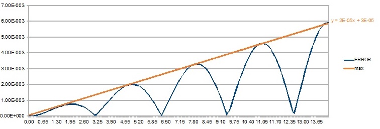
The variation of the position of an atom was calculated using the classical harmonic oscillator approach and the Velocity-Verlet algorithm. Image 1 shows the difference between the two methods.

The orange line traces de maximum error peaks. It can be seen that these maximum errors increase linearly ($y=2*10^{-5}x+3*10^5$) with time. The reason behind this is that the simulation of each time-step requires that of the previous one, so the error builds up. Tick. Be careful to check your grammar.

For the following simulations, since the energy of an ensemble should be constant over time we needed to find the value of the time-step that would give the lowest standard deviation in order words, the least energy fluctuations. The following table shows that 0.03 gives a 1% STD. Tick although I don't think your table does explicitly show this

Energy Fluctuation with time.

Time-step	Standard deviation
0.1	0.18
0.01	0.17
0.001	0.003
0.002	0.012

Task 4: Lennard Jones Potential:

• Finding $r_0$ at which the potential is zero:

$\varphi \left(r\right)=4ϵ(\frac{{\sigma }^{12}}{r^{12}}-\frac{{\sigma }^6}{r^6})$

Since $\varphi \left(r_o\right)=0$:

$4ϵ(\frac{{\sigma }^{12}}{r_0^{12}}-\frac{{\sigma }^6}{r_0^6})=0$

And:

$\frac{{\sigma }^{12}}{r_0^{12}}=\frac{{\sigma }^6}{r_0^6}$

${\sigma }^6{r}_0^{12}={\sigma }^{12}{r}_0^6$

$\frac{{\sigma }^6}{{\sigma }^{12}}=\frac{r_0^6}{r_0^{12}}$

$\frac{1}{{\sigma }^6}=\frac{1}{r_0^6}$

${\sigma }^6=r_0^6$

Finally $\sigma =r_0$ Tick

• Force at seperation at $r_0$ equal to $\frac{d(\varphi \left(r_0\right))}{d{r}_0}$

$\frac{{\sigma }^6}{{\sigma }^{12}}=\frac{r_0^6}{r_0^{12}}$

$F=\frac{-4ϵ{\sigma }^{12}12}{r_0^{13}}+\frac{4ϵ{\sigma }^{6}6}{r_0^7}$

$F=\frac{-48ϵ{\sigma }^{12}}{r_0^{13}}+\frac{24ϵ{\sigma }^6}{r_0^7}$

Since $\sigma =r_0$ at this point,

$F=\frac{-48ϵr_0^{12}}{r_0^{13}}+\frac{24ϵr_0^6}{r_0^7}$

$F=\frac{-48ϵ+24ϵr_0^6}{r_0^7}$

$F=\frac{-24ϵ}{r_0}$ or $F=\frac{-24ϵ}{\sigma }$ Tick.

• Finding the equilibrium separation:

The equilibrium separation $r_{eq}$ corresponds to the energy minimum of the Lennard Jones potential curve. As it is the minimum it will be a solution of equating the first derivative of $\varphi \left(r\right)$ to zero.

Calculating $\frac{d(\varphi \left(r\right))}{dr}$ and knowing it has to equal to zero.

$\frac{d(\varphi \left(r\right))}{dr}=\frac{-48ϵ{\sigma }^{12}}{r^{13}}+\frac{24ϵ{\sigma }^6}{r^7}$ = $\frac{-48ϵ{\sigma }^{12}{r}^7}{r^{20}}+\frac{24ϵ{\sigma }^6{r}^{13}}{r^{20}}$ = $\frac{-48ϵ{\sigma }^{12}{r}^7+24ϵ{\sigma }^6{r}^{13}}{r^{20}}$

$\frac{-24ϵ{\sigma }^6{r}^7(-2{\sigma }^6+r^6)}{r^{20}}=0$

$(-2{\sigma }^6+r^6)=0$

$2{\sigma }^6=r^6$

$r_{eq}=\sqrt[6]{2}\sigma$' Tick.

• Now the well depth can be found

$\varphi (r_{eq})=4ϵ(\frac{{\sigma }^{12}}{{\sqrt[6]{2}}^{12}{\sigma }^{12}}-\frac{{\sigma }^6}{{\sqrt[6]{2}}^6{\sigma }^6})$ = $4ϵ(\frac{1}{2^2}-\frac{1}{2})$ =$4ϵ(\frac{-1}{4})$=$-ϵ$ Tick

• Evaluating integrals $\underset{2\sigma }{\overset{\mathrm{\infty }}{\int }}\varphi \left(r\right)\mathrm{d}r$, $\underset{2.5\sigma }{\overset{\mathrm{\infty }}{\int }}\varphi \left(r\right)\mathrm{d}r$, and $\underset{3\sigma }{\overset{\mathrm{\infty }}{\int }}\varphi \left(r\right)\mathrm{d}r$. With values of $\sigma =ϵ=1.0$

$\underset{2\sigma }{\overset{\mathrm{\infty }}{\int }}\varphi \left(r\right)\mathrm{d}r=\underset{2\sigma }{\overset{\mathrm{\infty }}{\int }}\mathrm{4}\mathrm{ϵ}(\frac{{\sigma }^{12}}{r_0^{12}}-\frac{{\sigma }^6}{r_0^6})\mathrm{d}r=[\frac{1}{4}(-\frac{{\sigma }^{12}}{11*2^{11}{\sigma }^{11}}+\frac{{\sigma }^6}{5*2^5{\sigma }^5}){]}_{2\sigma }^{\mathrm{\infty }}$ = $\frac{1}{4}(-\frac{1^{12}}{11*2^{11}{1}^{11}}+\frac{1^6}{5*2^5{1}^5})=-0.0248$

The same process was followed for the other integrals:

$\underset{2.5\sigma }{\overset{\mathrm{\infty }}{\int }}\varphi \left(r\right)\mathrm{d}r=-\frac{1}{4}ϵ(-\frac{{\sigma }^{12}}{11*2.5^{11}{\sigma }^{11}}+\frac{{\sigma }^6}{5*2.5^5{\sigma }^5})=-0.00818$

$\underset{3\sigma }{\overset{\mathrm{\infty }}{\int }}\varphi \left(r\right)\mathrm{d}r=-\frac{1}{4}ϵ(-\frac{{\sigma }^{12}}{11*3^{11}{\sigma }^{11}}+\frac{{\sigma }^6}{5*3^5{\sigma }^5})=-0.00329$ Tick. Good

Task 5: Number of water molecules in 1ml of water and volume of 1000 water molecules

1mL of water equals 1 gr of water. Dividing this gram by 18.01528 g/mol, the molar density of water we get 0.0555 mol of water. Finally by multiplying by Avogadro's number we find that there are $3.3422810^{22}$ molecules of water in 1 mL.

Proportionally, 10000 molecules will occupy a volume of $2.991*10^{-19}$ mL. Tick.

Task 6:

An atom at position $(0.5,0.5,0.5)$ sits in a cubic simulation box of dimensions from $(0,0,0)$ to $(1,1,1)$ with periodic boundary conditions. If this atom moves along the vector $(0.7,0.6,0.2)$ it will end up at $(0.2,0.1,0.7)$. Tick.

Task 7: Reduced Units

The Lennard-Jones parameters for argon are $$\begin{gathered} \sigma =0.34\mathrm{n}\mathrm{m},ϵ \\ / \\ {k}_B=120\mathrm{K} \end{gathered}$$. If the LJ cutoff is $r^{*}=3.2$, what is it in real units? What is the well depth in $$\begin{gathered} {\mathrm{k}\mathrm{J} \\ \mathrm{m}\mathrm{o}\mathrm{l}}^{-1} \end{gathered}$$? What is the reduced temperature $T^{*}=1.5$ in real units?

$r=1.088$' Tick. Units?

$T=180K$ Tick.

$$\begin{gathered} ϵ \\ =0.014{kJ \\ mol}^{-1} \end{gathered}$$ Not quite - you used the Lennard-Jones parameter?

Task 8: Density and lattice spacing

Using the formula for density:

$\rho =\frac{m}{V}$$=\frac{1}{1.077^3}$$=0.79999\approx 0.8$ Tick.

If we consider a fcc lattice, (4 atoms per unit cell), with density of 1.2 and using the formula above:

$1.2=\frac{4}{x^3}$

Where x is the side length of a unit cell

$x=\sqrt[3]{\frac{4}{1.2}}\approx 1.275$ Tick.

Why do random coordinates cause problems in simulations? Two overlapping atoms results in large forces. Larger forces require smaller timesteps

Task 9 Number of atoms with an fcc lattice

With the established set-up, 1000 unit cells are created. If an fcc lattice had been chosen 1000 unit cells would have also been formed each containing 4 atoms which add up to a total of 4000 atoms. Tick.

Task 10: Input script commands.

The commands are used to determine the properties of the atoms.

 mass 1 1.0

Sets the mass for all atoms of type 1 to a value of 1.0. Tick. In what units? It is worth remembering that for this simulation only 1 atom type has been used.

pair_style lj/cut 3.0

Calculates the coulombic pairwise interaction of two neighbouring atoms as the distance increases between them until a maximum of 0.3 in the Lennard-Jones potential. Tick. Units?

pair_coeff * * 1.0 1.0

Specifies the pairwise force field coefficients between atoms pairs. The asterisks indicate that all atoms types from 1 to N will have a value of 1. More detail would be good here. The asterisks tell LAMPPS that this command applies to "all atoms and atom types". The two numbers represent sigma and epsilon

Task 11: Integration algorithm

By specifying ${\mathbf{x}}_i\left(0\right)$ and ${\mathbf{v}}_i\left(0\right)$, we are using the Velocity-Verlet algorithm. Tick.

Task 12: Understanding the code

variable timestep equal 0.001
variable n_steps equal floor(100/${timestep})
variable n_steps equal floor(100/0.001)
timestep ${timestep}
timestep 0.001

The code above is used to constrain the number of steps depending on the time-step. This is easily visualized by choosing two different time-steps:

timestep equal 0.001 $⟹$ n_steps = 100000

timestep equal 0.002 $⟹$ n_steps = 50000

The two time-steps have different number of steps but the sum of the time-steps is constant and its 100.

In other words, the number of $\delta t$'s in the Velocity Verlet algorithm is different but their sum is constant.

This sum of the time-steps is not dependent on the actual duration of the simulation. Ok. However, this was more asking about the purpose of the timestep variable. Just like programming, variables allow you to change a value throughout your code simply

Task 13: Variation of Energy, Pressure and Temperature plots with the time-step.

Tick.

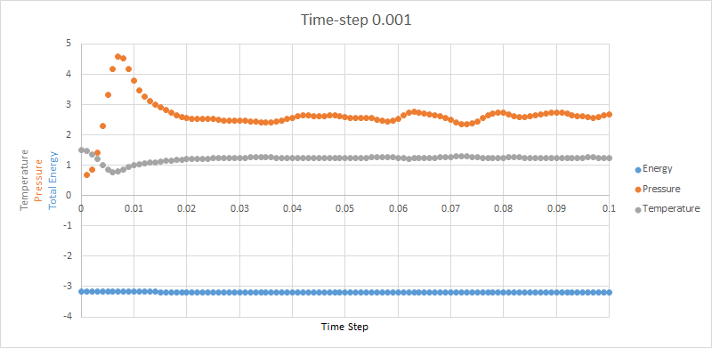
It can be seen from Image that for a 0.001 times-step the simulation reaches equilibrium at around 0.02. Although pressure and temperature fluctuate throughout the simulation the energy remains constant with a standard deviation of___ that was previously calculated.This result was therefore expected. Be careful to go through your report and check you've filled in all your blanks

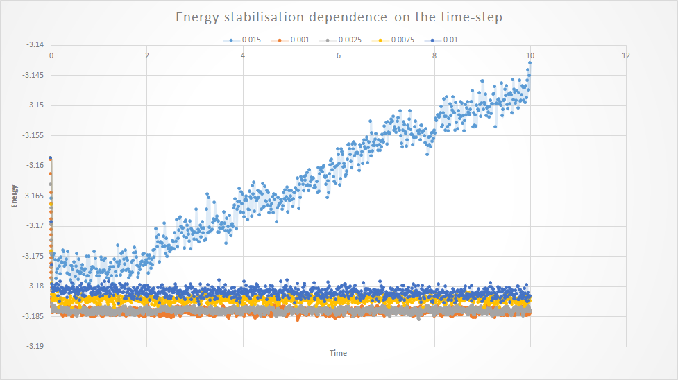
If we know *typo compare the effect of the time-step on the energy the following conclusions can be drawn:

• The larger the time-step, the less accurate the Velocity-Verlet algorithm, choosign *typo a larger time-step causes the error to increase
• Both 0.001 and 0.0025 give accurate energy readings but choosing 0.0025 will allow the simulations to run for longer.
• Above 0.003 The standard deviation of the energy increases to
• 0.015 as a time step does not reach an energy stabilisation.
  

In view of the above, the simulations will be run for both 0.001 and 0.0025 as time-steps. Accuracy vs. computational efficiency. You want a small timestep but you want a timestep that requires less time to run

Task 14: Determining $\gamma$

$\frac{1}{2}\sum _i{m}_i{v}_i^2=\frac{3}{2}N{k}_{B}T$

To achieve $T=\mathfrak{𝔗}$ every $v_i$ has to be multiplied by $\gamma$

$\frac{1}{2}\sum _i{m}_i{\left(\gamma v_i\right)}^2=\frac{3}{2}N{k}_B\mathfrak{𝔗}$

$$\begin{gathered} {\gamma }^2\frac{1}{2}\sum _i{m}_i{\left( \\ {v}_i\right)}^2=\frac{3}{2}N{k}_B\mathfrak{𝔗} \end{gathered}$$

Substituting $\frac{1}{2}\sum _i{m}_i{v}_i^2$:

${\gamma }^2\frac{3}{2}N{k}_{B}T=\frac{3}{2}N{k}_B\mathfrak{𝔗}$

Cancelling and rearranging leads us to:

$\gamma =\sqrt{\frac{\mathfrak{𝔗}}{T}}$ Tick

Task 15: Numbers 100 1000 100000

• First: Use the input values every this number of time steps.
• Second: number of times to repeat the input values for calculating the averages.
• Third: To calculate averages for this frequency of timesteps

Task 16: Editing the equations of state

Ensure that your graphs have an appropriate legend if you have more than one graph on the same plot

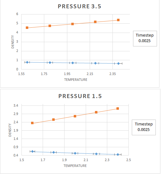
The graphs above show the change in density with respect to temperature. These simulations of ensembles were run at a time-step of 0.0025 that as shown in Task 1 ensures that the energy of the system does not fluctuate more than 1%. From these graphs several conclusions can be drawn:

- An increase in temperature causes a decrease in density.

- An increase in pressure causes an increase in density.

What about your calculated densities vs. the ideal gas? How does the discrepancy change with temperature?

Task 17: Heat Capacities

For this simulation a file was created File:Log file.rtf

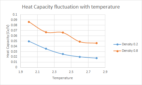
From the plot above it can be seen that a temperature increase causes a decrease in heat capacity. <span style="color:red"Tick.

The reasoning behind this trend is that because the simulation establishes a certain lattice structure there is a constraint on the positions of the atoms. This constraint stops the atoms from gaining free energy. At constant volume the heat capacity can be written as $C_V=(\frac{dU}{dT}{)}_V$ . Consequently if the increase in internal energy is not greater that the temperature increase the heat capacity will decrease. Nice idea but think about the density of states and how it changes with an increase in temperature

A change in density changes the volume of the lattice cells, as calculated in Task . Be careful to go through your report and check you've filled in all your blanks At higher densities the heat capacity of the system increases. This is due to the lattice cells being more effectively filled and hence more atoms per area can potentially increase their internal energy.

Task 18: Radial distribution functions

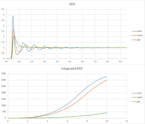
The radial distribution plots for solid, liquid and gas can be seen below.

For this simulation, a face centred cubic lattice was used and the values for the density and temperature were chosen according to the phase diagram of a Lennard-Jones system.

All plots start at zero as the potential interaction, which an atom experiences from others at a position x=0 from itself, is zero.

As the distance from that atom is increased there is an increasing probability of encountering other atoms.

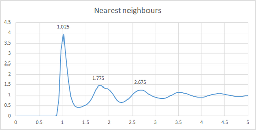
In a gas, due to the free motion of the atoms around the simulation box, the RDf RDF stands for radial distribution function function goes the fastest to zero. For the liquid as there is a reduce *Typo in motion and an increase of the atoms to be fixed to the lattice structure the first peak quickly flattens out. What about the peaks? Finally, for a solid, due to the fixed nature of the atoms to the lattice sites, the RDF peaks can be related to the distance to the nearest neighbours, which in this case are 1.025, 1.775 and 2.675 as shown on the plot below.

From the looks of your RDF, you simulated a liquid for your solid plot. Additionally, would be nice to discuss the long-range order in each and compare to their RDFs

Some more description here would be good. In the solid case, illustrate which lattice distances correspond to the first three peaks. What is the lattice spacing in the solid? What is the coordination number for each of the first three peaks in the solid?

Task 19: Mean Squared Displacement

The MSD was plotted as seen on the images on the right. Fronm those plots, the gradient was calculated and divided by 6 to give D, the diffusion coefficient. the results are summarized in the following table:

D from MSD plots.

	Solid	Liquid	Gas
Millions	8.33E-9	1.66E-4	0.005
fcc	1.16E-9	0.0011	0.00303
sq lat	3.3E-6	0.0011	0.00302

There are two trends than can be inferred from the MDS plots.

• The diffusion coefficient increases when going from a solid phase to a liquid or a gas.
• The greater the density of the lattice, fcc with 4 atoms per simulation box, the lower the diffusion coefficient.

Under the same density conditions of the ensemble, the intrinsic density of an square lattice with 1 atom per simulation box, causes it to have an MSD plot which resembles after a liquid more than after a solid. Typos. Tick

VACF?

References

Peter Atkins, Julio de Paula, Atkins Physical Chemistry, Oxford 2008.

Hansen, J.-P., & Verlet, L. (1969). Phase Transitions of the Lennard-Jones System. Phys. Rev., 184(1), 151–161. http://doi.org/10.1103/PhysRev.184.151