Talk:Mod:AC2015LQ

JC: General comments: Good answers to most tasks, but a few tasks missing or not completed towards the end. Try to check through your work at the end to make sure that it is clear and complete.

Liquid Simulations

Background and Introduction to Molecular Dynamics

Molecular dynamics simulations are used in this report to calculate thermodynamic properties of various ensembles. The LAMMPS code was utilised to write these calculations, and they were subsequently performed on the University High Performance Computing (HPC) facilities. There is much history of using large HPC systems (e.g. ARCHER) to measure properties of large data sets, but many approximations must be made.

Here it is assumed that atoms behave as classical particles governed by Newton's Second Law, i.e. $F=ma$

This can be adapted to allow a simulation of atomic movement over time - the essence of molecular dynamics simulations. Of course if we were to simulate every individual atom there would be a huge expense in terms of computer processing energy and thus the velocity Verlet algorithm is implemented to give a good approximation to the overall system.

Initial simulations were run to find the timestep to be used in subsequent calculations.

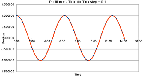
The file HO.xls provided data for the position $x$, velocity $v$ and force $f$ of a system across a range of time. This may be used to model the behaviour of a classical harmonic oscillator using the velocity-Verlet algorithm mentioned previously. The behaviour was also modelled using the classical method and good agreement between the models visible in Figure 1

Figure 1

Energies

The energy of the system was calculated from a summation of the potential and kinetic energies:

$E=E_{kinetic}+E_{potential}=K+U=\frac{1}{2}m{v}^2+\frac{1}{2}k{x}^2$

where $m$ is mass (given as 1.00), $v$ is velocity and $k$ is the force constant (given as 1.00)

Energy must be conserved for the simulation to provide a physically valid model (as per Newton's Third Law). However there is an inherent error in molecular dynamics calculations (due to the approximations that must be made link to later approxs). Hence the energy calculated with MD simulations drifts in accordance with Brownian motion .

JC: Checking conservation of energy is a way to check the validity of a simulation.

The velocity-Verlet simulation used does not conserve energy but instead keeps it fluctuating about a constant value over long periods of time. Hence the optimal timestep will give a minuscule variation in energy, but at the largest possible timestep to save computational cost.

Timesteps were varied from 0.1 upwards, with the energies and the fluctuations listed in Table 1. The Energy versus Time Graph for a timestep of 0.1 is visible in Figure 2 below,

Figure 2

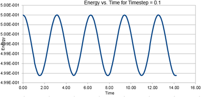
It was deduced that the simulations were valid for a timestep $\le$ 0.2.

This is because the average total energy of the oscillator for the velocity-Verlet solution is constant for each timestep at $E_{average}=0.5$

Hence to keep the energy within 1% required a fluctuation of less than or equal to 1% of 0.5:

$\mathrm{\Delta }E\le 0.5\times 10^{-3}$

Thus the maximum timestep to give an energy fluctuation of less than 1% was determined to be 0.2. (Timestep 0.21 gives a fluctuation greater than 0.5 (1%), with 0.205 also above 1%)

JC: Good thorough analysis of different timesteps and choice of 0.2.

Errors

It was also possible to calculate the error between the classical solution for the position at time $t$ and the position calculated using the velocity-Verlet algorithm, mentioned previously.

The classical solution was calculated using: $x\left(t\right)=A\cos (\omega t+\varphi )$

with $A=1.00$, $\omega =1.00$, and $\varphi =0$

The variation in absolute error between the two methods was calculated for the same timesteps as used to optimise the energy calculations. This error follows an envelope function, plotted linearly in Figures 3 and 4 for timesteps of $0.1$ and $0.2$.

Figures 3 and 4 - The Envelope Function showing the Error Maxima at timesteps 0.1 and 0.2 (L-R)

The variation in $x$ and $\mathrm{\Delta }E$ (both range and absolute) with timestep is summarised in Table 1, along with the number of error peaks. There is seen to be increasing error with deviation away from a suitable timestep (of $0.2$). This is rationalised in that more timesteps samples a longer period of time and hence there are more maxima on the error graphs.

Timestep	x max	x min	E max	E min	ΔE	Number of Error Peaks
0.1	1	-1	0.5	0.49875	0.00125	5
0.2	1	-1	0.5	0.49500	0.00500	9
0.21	1	-1	0.5	0.49449	0.00551	10
0.205	1	-1	0.5	0.49474	0.00525	9

Table 1

JC: Why does the error increase over time for any timestep?

Atomic Forces

The Lennard-Jones potential is used to model the interactions between pairs of atoms in our system. This simplifies the system to ignore Coulombic effects and simulates the potential energies of two uncharged molecules according to the curve shown in Figure 5, which has contributions from both positive attractions (due to the induced dipole moments of atoms moving in a liquid) and negative interactions (short-range repulsion between atoms).

Figure 5 - Potential Energy as a Function of r, Lennard Jones curve, Ref https://en.wikipedia.org/wiki/Melting-point_depression#/media/File:Lennard-Jones.jpg

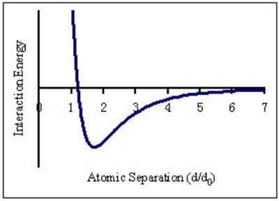
This is illustrated in the formula

$U\left({\mathbf{r}}^N\right)=4ϵ(\frac{{\sigma }^{12}}{r_{ij}^{12}}-\frac{{\sigma }^6}{r_{ij}^6})$

If the separation is small, the potential is dominated by the $\frac{{\sigma }^{12}}{r_{ij}^{12}}$ term - i.e. strongly positive, with much short-range repulsion.

As $r\mapsto \mathrm{\infty }$, the $\frac{{\sigma }^6}{r_{ij}^6}$ term dominates, hence long range attraction occurs.

Find the equilibrium separation, $r_{eq}$, and work out the well depth ($\varphi \left(r_{eq}\right)$). Evaluate the integrals $\underset{2\sigma }{\overset{\mathrm{\infty }}{\int }}\varphi \left(r\right)\mathrm{d}r$, $\underset{2.5\sigma }{\overset{\mathrm{\infty }}{\int }}\varphi \left(r\right)\mathrm{d}r$, and $\underset{3\sigma }{\overset{\mathrm{\infty }}{\int }}\varphi \left(r\right)\mathrm{d}r$ when $\sigma =ϵ=1.0$.

ANSWER:

• $r_0$ at which potential energy, $U$, equals 0:

It is clear that $U$ will become zero when $r_0=\sigma$ since this causes the term $\frac{{\sigma }^{12}}{r^{12}}-\frac{{\sigma }^6}{r^6}$ to equal 0.

As stated above, $r^{12}$ is long range repulsion; $r^6$ is long range attraction

• hence if $r_0=\sigma$ the force at this separation is calculated using

${\mathbf{F}}_0=-\frac{\mathrm{d}\varphi \left(\mathbf{r}\right)}{\mathrm{d}{\mathbf{r}}_0}$

${\mathbf{F}}_0=-\frac{\mathrm{d}U\left({\mathbf{r}}^N\right)}{\mathrm{d}{\mathbf{r}}_i}$

• and since

$U\left({\mathbf{r}}^N\right)=\sum _i^N\sum _{i\ne j}^N\left\{4ϵ(\frac{{\sigma }^{12}}{r_{ij}^{12}}-\frac{{\sigma }^6}{r_{ij}^6})\right\}$

The force at $U=0$ is equal to:

${\mathbf{F}}_0=0-\sum _i^N\sum _{i\ne j}^N\left\{4ϵ(\frac{{\sigma }^{12}}{r_{ij}^{12}}-\frac{{\sigma }^6}{r_{ij}^6})\right\}$ $=4ϵ\frac{12{\sigma }^{12}}{r_0^{13}}-\frac{6{\sigma }^6}{r_0^6}$

Giving

${\mathbf{F}}_0=\frac{24ϵ}{\sigma }$

the separation at equilibrium $r_{eq}$ has a force equal to zero:

${\mathbf{F}}_{eq}=-\frac{\mathrm{d}\varphi \left(\mathbf{r}\right)}{\mathrm{d}{\mathbf{r}}_{\mathbf{e}\mathbf{q}}}=0$

thus

$\frac{12{\sigma }^{12}}{r_{eq}^{13}}-\frac{6{\sigma }^6}{r_{eq}^7}$

$2{\sigma }^6=r_{eq}^6$

$r_{eq}=\sigma 2^{\frac{1}{6}}$

and

$\varphi (r)=4ϵ(\frac{{\sigma }^{12}}{2^2{\sigma }^{12}}-\frac{{\sigma }^6}{2{\sigma }^6})$

$=4ϵ(\frac{1}{4}-\frac{1}{2})$

Hence

$\varphi (r)=-ϵ$

The integrals given may then be evaluated by setting $\sigma =ϵ=1.0$:

• $\underset{2\sigma }{\overset{\mathrm{\infty }}{\int }}\varphi \left(r\right)\mathrm{d}r=-0.025$

• $\underset{2.5\sigma }{\overset{\mathrm{\infty }}{\int }}\varphi \left(r\right)\mathrm{d}r=-0.008$

• $\underset{3\sigma }{\overset{\mathrm{\infty }}{\int }}\varphi \left(r\right)\mathrm{d}r=-0.003$

JC: All maths correct and nicely presented.

Periodic Boundary Conditions

Using the velocity-Verlet algorithm all we must define is the initial starting positions and velocities.

These simulations are performed for $N$ between $1000$ and $10000$ since it is too expensive to simulate realistic volumes.

The number of water molecules in 1ml of water under standard conditions may be estimated as follows:

• $pressure=P=10^{5}Pa$
• $temperature=T=273.15K$
• $concentration=c^o=1mold{m}^{-3}$

$1ml{H}_{2}O=1d{m}^3$

JC: Careful with units and volumes, 1 ml = 1e-3 dm3 and in the next line your conversion from kg m-3 to g dm-3 is also out by 1e3, however, the errors cancel in the end so your answer is correct.

$densityof{H}_{2}O=\rho =999.8395kg{m}^{-3}=0.998395gd{m}^{-3}$ under standard conditions

therefore mass of $1d{m}^3=0.998395gd{m}^{-3}\times 1d{m}^3=0.998395g$

since $mass(H_{2}O)=18.015gmo{l}^{-1}$, number of molecules of $H_{2}O=\frac{0.998395g}{18.015gmo{l}^{-1}}\times N_A=3.35\times 10^{22}mol$

To estimate the volume of $10000$ water molecules under standard conditions:

the volume of one molecule may be deduced from the first calculation above:

$volume(onemolecule)=\frac{totalvolume}{numberofmolecules}$

thus:

$volume(onemolecule)=\frac{volume(3.35\times 10^{22}mol)}{3.35\times 10^{22}mol}=\frac{1d{m}^3}{3.35\times 10^{22}mol}=2.99\times 10^{-23}d{m}^{-3}$

and so the volume of $10000$ molecules is simply:

$10000\times 2.99\times 10^{-23}d{m}^{-3}=2.99\times 10^{-19}d{m}^{-3}$

We utilise a periodic box (similar to a unit cell) to generate a system of large volume. If an atom leaves at one position, its replica will enter from the opposite direction.

Consider an atom at position $(0.5,0.5,0.5)$ in a cubic simulation box which runs from $(0,0,0)$ to $(1,1,1)$. In a single timestep, it moves along the vector $(0.7,0.6,0.2)$. It therefore ends up at the point $(0.2,0.1,0.7)$

JC: Correct.

Because..:

$0.5+0.7=1.2$ which becomes $0.2$ in this system of volume $(0,0,0)$ to $(1,1,1)$

$0.5+0.1=0.6$ o.k. / within cube boundaries

JC: Should this be 0.5 + 0.6?

$0.5+0.2=0.7$ fine also within the boundaries

Reduced Units

We simplify the calculations performed in the Lennard-Jones simulation by using reduced units, denoted by a star

e.g. distance $r$ becomes $r*$.

The Lennard-Jones parameters for argon are $$\begin{gathered} \sigma =0.34\mathrm{n}\mathrm{m},ϵ \\ / \\ {k}_B=120\mathrm{K} \end{gathered}$$.

• LJ cutoff:

$r^{*}=3.2=\frac{r}{\sigma }$

Therefore

$r=r^{*}\sigma =3.2\times 0.34nm=1.088nm$ ~ $1.09nm=1.09\times 10^{-9}m$

• well depth:

$ϵ=120k_B=120K\times 1.3806\times 10^{-23}J{K}^{-}1=1.657\times 10^{-21}J$

therefore per molecule the well depth is:

$1.657\times 10^{-21}J/N_A=1.66\times 10^{-21}J/6.0221\times 10^{23}kJmo{l}^{-1}=1.66\times 10^{-24}\times 6.0221\times 10^{23}kJmo{l}^{-}1=1.0kJmo{l}^{-1}$

• the reduced temperature:

$T^{*}=\frac{k_{B}T}{ϵ}=\frac{k_{B}T}{k_B\times 120K}$

When $T^{*}=1.5$ ,this rearranges to:

$T=\frac{1.5\times k_B\times 120K}{k_B}=1.5\times 120K=180K$

JC: Good conversion of reduced units.

Equilibration

The Simulation Box

Using the velocity-Verlet algorithm required the initial starting conditions to be set. This is fairly straightforward for a crystal in which the lattice parameters are known, but for a liquid without fixed bonds it requires a different approach.

If the positions of atoms were simply picked at random, a physically impossible system may be generated, in which atoms co-exist in the same region of space. Clearly it is impossible for two (or more) atoms to overlap with one another - the fact they are physical objects makes this so.

JC: Why can atoms not overlap? Placing atoms at random can lead to configurations with very high repulsion between atoms which can make the system unstable.

This is illustrated by the Lennard-Jones curve where $E_{pot}\mapsto \mathrm{\infty }$ as $r\mapsto 0$

The lattice spacing in the LAMPPS is output as

Lattice spacing in x,y,z = 1.07722 1.07722 1.07722

This gives a number density $=0.8$ shown by the following calculations:

(Knowing that for a cubic lattice we have one lattice point per unit cell)

$numberdensity(\rho )=\frac{numberoflatticepoints}{volumeof3Dlattice}$

lattice spacing $d=1.07722$

$d^3=1.07722^3=1.250009243$

$\rho =1/d^3=0.799999\approx 0.8$

A face-centred cubic lattice with a lattice point number density of 1.2 has a unit cell side length of $\approx 1.49$

This is calculated as follows:

$(\frac{4}{1.2}{)}^{\frac{1}{3}}=3.3333333^{\frac{1}{3}}=1.493801582$

The

create_atoms

command defines the number of atoms created for a lattice.

For a simple cubic cell there is 1 lattice point per unit cell, whilst a face centred cubic cell has 4 lattice points per unit cell.

Therefore 1000 unit cells will have 1000 atoms for a sc system but 4000 atoms for an fcc system.

JC: Correct answers clearly shown.

LAMMPS and syntax

The input script contains the following commands:

• mass 1 1.0
• pair_style lj/cut 3.0
• pair_coeff * * 1.0 1.0

mass 1 1.0

This sets the mass of atom 1 (for a given atom of pure fluid) set to equal a value of 1.0

pair_style lj/cut 3.0

This sets the cutoff point (at which we no longer have atoms pairing with each other) to the Lennard-Jones (lj) potential, and since atoms are not bonded to each other in this system, this also defines which neighbouring atoms are & aren't interacting. Hence nearest neighbours and pairing potentials vary over time.

pair_coeff * * 1.0 1.0

This defines the pairwise force field coefficients; the leading asterisk and trailing asterisk combine to give all atom types from 1 to n and n to N which in this instance is simply 1 (as there is only 1 type of atom). Hence also the atom coefficients in a pair are both set to 1.0 since the atoms are of the same type and so have equal contributions to a pairwise force field. The final term sets the coefficients for all atom pairs to equal 1.

JC: What are the atom coefficients?

The simulation now has 1000 atoms, with the starting position $t=0$, masses and interatomic forces defined for each of them.

The final thing we need to define to completely specify the initial conditions is the velocity of each atom. The velocities of atoms in any system are defined by the Maxwell-Boltzmann distribution - this is easily achieved for

all

atoms at a reduced temperature of

1.5

using LAMPSS with the script

 velocity all create 1.5 12345 dist gaussian rot yes mom yes 

Given that we are specifying $xi(0)$ and $vi(0)$ , we use the velocity-Verlet algorithm in our simulations.

Specifying the timestep

The script includes the lines

 
### SPECIFY TIMESTEP ###
variable timestep equal 0.001 

It is written in this way since we want to use different values of timesteps (0.001, 0.0025, 0.0075, 0.01 and 0.015) to calculate the same measurements. If we simply used

timestep 0.001
 run 100000

it would not be possible to simply alter the code in future calculations with a different timestep (variable).

Moreover if we want to calculate the same overall time for different numbers of steps the floor function enables this.

JC: Defining a variable called timestep means that we can use the value of the variable in other commands and calculations throughout the script, so to change the timestep, only the value of the variable needs to be changed.

Some screengrabs showing VMD simulation progress for 2 molecules singled out of the system

The spheres modeled in VMD may change position across the box very rapidly when it reaches one periodic boundary, and is reflected back across the other face

JC: Number the figure and then you can refer to it in the text.

Checking Equilibration

Simulations were visualised using VMD software to determine whether equilibrium was reached - and whether it was reached to a suitable degree of accuracy. This allows the determination of a suitable timestep for calculations that will be performed later on.

The simulation reached equilibrium for the four smallest timesteps, as visible by the plateaus in Figure 6. However the largest timestep of 0.015 failed to bring the system to equilibrium and therefore definitely should not be used.

Figure 6 - Energy versus Time for all the timesteps

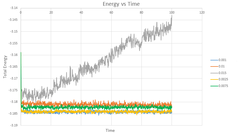
Thus timesteps 0.001, 0.0025, 0.0075 and 0.01 give reasonable results as they all reach equilibrium. However it is clear that the measurements are less accurate above the timestep of 0.0025, since the energy oscillates at a higher energy. The timestep of 0.0075, has a 0.06% error in energy with respect to the energy calculated at a timestep of 0.001 (the smallest and therefore most accurate system), which increases to 0.1% for ts = 0.01. In terms of cost, 0.0025 requires 40000 steps whilst 0.0075 requires 1334 steps. There is not a huge computational cost to improving the accuracy - thus the timestep of 0.0025 (with % error for energy = 0.005) is the best compromise between accuracy and cost.

JC: Good choice of timestep.

To determine how long the system took to reach equilibrium, the plots of Energy versus Time for a timestep of 0.001 were zoomed in. It is apparent that equilibrium is reached at a time of roughly 0.5.

Figure 7 -Zooming into the graph to see at what point the system reaches equilibrium

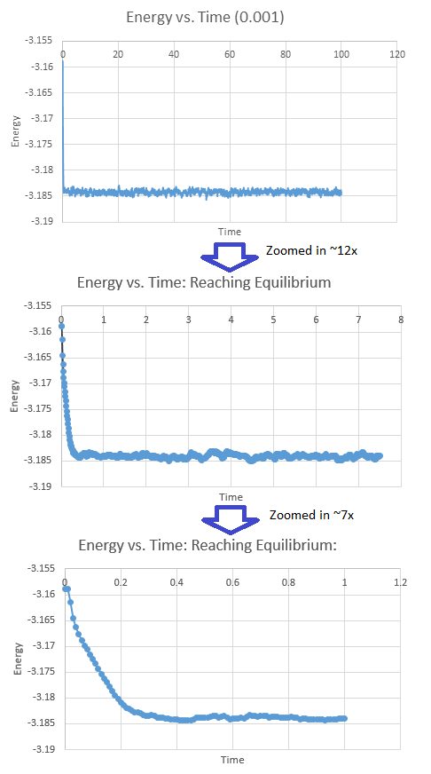
It is also apparent that equilibrium conditions were reached by inspection of the Pressure-Time and Temperature-Time plots, seen in the Figures 8 and 9. The results for the other timesteps were consistent with these, and validates the choice of 0.0025 for further calculations.

Figure 8 - Pressure versus Time for the 0.001 Timestep

Figure 9 - Temperature versus Time for the 0.001 Timestep

JC: Good analysis to see the simulation reaching equilibrium over time based on pressure and temperature.

Running Simulations under Specific Conditions

The simulations thus far were performed using the microcanonical (NVE) ensemble, and seen to give a constant average value for timesteps of less than 0.01.

However to investigate thermodynamic properties under specific conditions, the isobaric-isothermal ensemble (NpT) must be employed instead. This ensemble keeps the temperature and pressure constant, and again uses a defined timestep to model the simulation. The optimal timestep has already been chosen as 0.0025.

Ten simulations were run with the following parameters (Shown in Table 2) (in reduced units):

Pressure	Temperature
2.5	1.55
2.5	1.65
2.5	1.75
2.5	1.85
2.5	1.95
2.7	1.55
2.7	1.65
2.7	1.75
2.7	1.85
2.7	1.95

Table 2

The pressures were chosen to be close to the average pressure of 2.62 from the equilibrium simulations. This should give a physically reasonable system. From these ten simulations, ten phase points are generated from which an Equation of State may be derived.

Thermostats and Barostats

The equipartition theorem states that, on average, every degree of freedom in a system at equilibrium will have $\frac{1}{2}{k}_{B}T$ of energy. In our system with $N$ atoms, each with 3 degrees of freedom, we can write

$E_K=\frac{3}{2}N{k}_{B}T$

$\frac{1}{2}\sum _i{m}_i{v}_i^2=\frac{3}{2}N{k}_{B}T$

At the end of every timestep, we use the left hand side of this equation to calculate the kinetic energy, then divide by $\frac{3}{2}N{k}_B$ to get the instantaneous temperature $T$. In general, $T$ will fluctuate, and will be different to our target temperature, $\mathfrak{𝔗}$. We can change the temperature by multiplying every velocity by a constant factor, $\gamma$.

• If $T>\mathfrak{𝔗}$, then the kinetic energy of the system is too high, and we need to reduce it. $\gamma <1$
• If $T<\mathfrak{𝔗}$, then the kinetic energy of the system is too low, and we need to increase it. $\gamma >1$

We need to choose $\gamma$ so that the temperature is correct $T=\mathfrak{𝔗}$ if we multiply every velocity $\gamma$. We can write two equations:

$\frac{1}{2}\sum _i{m}_i{v}_i^2=\frac{3}{2}N{k}_{B}T$

$\frac{1}{2}\sum _i{m}_i{\left(\gamma v_i\right)}^2=\frac{3}{2}N{k}_B\mathfrak{𝔗}$

These may be solved to determine $\gamma$:

Since $T=\mathfrak{𝔗}$, $\frac{T}{\mathfrak{𝔗}}=1$

Thus

$\frac{\frac{1}{2}\sum _i{m}_i{v}_i^2}{\frac{1}{2}\sum _i{m}_i{\left(\gamma v_i\right)}^2}=1$

If we expand $(\gamma v_i{)}^2$ to ${\gamma }^2{v}_i^2$, the fraction becomes:

$\frac{\sum _i{m}_i{v}_i^2}{\sum _i{m}_i\left({\gamma }^2{v}_i^2\right)}=1$

hence

$\gamma =(1{)}^{\frac{1}{2}}$

or substituting back in the relationship $\frac{T}{\mathfrak{𝔗}}=1$

the factor is equal to:

$\gamma =(\frac{T}{\mathfrak{𝔗}}{)}^{\frac{1}{2}}$

JC: Correct final expression, but don't substitute T/(target T) = 1 in your derivation.

Examining the Input Script

The temperature and pressure are controlled by the line:

fix aves all ave/time 100 1000 100000 v_dens v_temp v_press v_dens2 v_temp2 v_press2

This translates to:

• fix = operation
• aves all = group of atoms this operation is being applied to (all atoms here)
• ave/time = style name of this command
• 100 = use input values every this many timesteps (every 100 timesteps)
• 1000 = number of times to use input values for calculating averages (1000 since 1000 atoms)
• 100000 = calculate averages every this many timesteps (just once in this simulation then since overall sim is 100000 timesteps)

Hence the average is calculated for the whole system, with the parameters being sampled every 100 timesteps (which equals 100000/100 = 1000 times) and (100000/1000=)100 measurements contributing to the average. The amount of time simulated is (100000*0.0025 =) 250 (in reduced units).

Plotting the Equations of State

Figure 10 - Density versus Temperature at both pressures

JC: There seems to be very little difference between the simulated results in the two graphs above.

The density ($\frac{N}{V}$) at each pressure was plotted as a function of temperature, and is visible via a blue line in Figure 10. The error bars shown correspond to the standard error associated with each phase point, as detailed in the output log file. The vertical error bars are too small to be seen on the graphs since the error in density was in the order of $3\times 10^{-3}$

The density may be calculated from the ideal gas law using $\rho =\frac{N}{V}$

$PV=nRT=N{k}_{B}T$ with the number of moles of gas $n=\frac{N}{N_A}$ and the gas constant $R=N_A{k}_B$

hence

$\rho =\frac{N}{V}=\frac{P}{k_{B}T}$

In reduced units, $k_B=0$ and hence the density is easily calculated from the pressure and temperatures as shown by the orange line in the Density-Temperature graphs in Figure 10.

JC: In reduced units $k_B=1$.

The ideal gas law predicts a higher density than that simulated. This was anticipated because the ideal gas law holds assumptions that neglect atom size and interatomic attractions, thus placing atoms at distances further apart than they are in reality.

However, at higher pressure, the average distance between atoms is less significant with respect to molecular size and so the neglection of atom size becomes less important, and the ideal gas model becomes more accurate. Similarly, at higher temperatures the neglection of interatomic attractions is less important (since they are reduced) and again, the two models are closer in value.

JC: Do you expect the ideal gas to be a good approximation for gases at high or low pressures?

As the temperature increases, the atoms gain more energy and thus are separated by a greater distance (increased repulsion) and thus the ideal gas model neglection of this distance becomes less important.

Hence the discrepancies between the ideal gas density and the simulated density decrease with both temperature and pressure. Mathematically, the average difference at $P=2.5$ is $0.746$, which reduces to $0.186$ at $P=2.7$.

Assumptions

• (1) N is very large (there is a large number of atoms), which obey Newton's laws of motion
• (2) the atomic volume is far smaller than the volume of the gas (negligible)
• (3) there are no forces (electrostatic or otherwise) acting on the atoms except extremely brief collisions (which are ignored)

Part 5 Heat Capacities of the System

The heat capacity $C_V$ of a system is defined by:

$C_V=\frac{\delta Q}{\delta T}$

For our system, the temperature is being held constant and thus we use fluctuations in the total energy to determine the capacity instead. The eqaution for this is:

$C_V=\frac{\partial E}{\partial T}=\frac{\mathrm{V}\mathrm{a}\mathrm{r}\left[E\right]}{k_B{T}^2}=N^2\frac{⟨E^2⟩-{⟨E⟩}^2}{k_B{T}^2}$

$\mathrm{V}\mathrm{a}\mathrm{r}\left[E\right]$ is the variance in $E$, $N$ is the number of atoms, and it is a standard result from statistics that $\mathrm{V}\mathrm{a}\mathrm{r}\left[X\right]=⟨X^2⟩-{⟨X⟩}^2$.

We use $N^2$ since we have calculated the energies in LAMMPS using the input script

 pair_style lj 

which normalises the energy by the number of atoms (i.e. the output $E$ is $\frac{E}{N}$

A script was written based on the file npt.in provided for the isobaric-isothermal ensemble. The differences made were:

• to allow the density of the system to be varied according to the

 sc 

lattice command syntax

• to change the NpT ensemble to NvT
• turn off the thermostat once the system has reached equilibrium (the crystal has melted)

• add variables to allow the calculation of the heat capacity, according to the equation above

• print the average temperature and heat capacity

plot $C_V/V$

$V=[latticeparameter{]}^3=1.07722^3=1.25001$

The plots are shown below

Figure 11

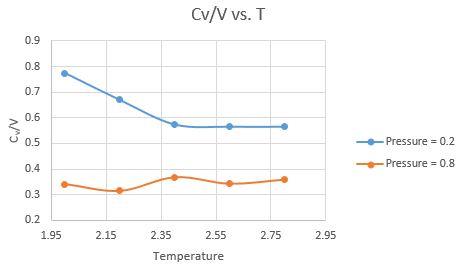
JC: Can you comment on this graph, what is the trend in heat capacity with temperature or density?

An example of the script used for $p=0.2,t=2.0$is:

### DEFINE SIMULATION BOX GEOMETRY ###
lattice sc 0.2
region box block 0 15 0 15 0 15
create_box 1 box
create_atoms 1 box

### DEFINE PHYSICAL PROPERTIES OF ATOMS ###
mass 1 1.0
pair_style lj/cut/opt 3.0
pair_coeff 1 1 1.0 1.0
neighbor 2.0 bin

### SPECIFY THE REQUIRED THERMODYNAMIC STATE ###
variable T equal 2.0 
variable p equal 2.5 
variable timestep equal 0.0025

### ASSIGN ATOMIC VELOCITIES ###
velocity all create ${T} 12345 dist gaussian rot yes mom yes

### SPECIFY ENSEMBLE ###
timestep ${timestep}
fix nve all nve

### THERMODYNAMIC OUTPUT CONTROL ###
thermo_style custom time etotal temp press
thermo 10

### RECORD TRAJECTORY ###
dump traj all custom 1000 output-1 id x y z

### SPECIFY TIMESTEP ###

### RUN SIMULATION TO MELT CRYSTAL ###
run 10000
unfix nve
reset_timestep 0

### BRING SYSTEM TO REQUIRED STATE ###
variable tdamp equal ${timestep}*100
variable pdamp equal ${timestep}*1000
fix nvt all nvt temp ${T} ${T} ${tdamp} 
run 10000
reset_timestep 0

unfix nvt 
fix nve all nve

### MEASURE SYSTEM STATE ###
thermo_style custom step etotal temp press density atoms
variable dens equal density
variable dens2 equal density*density
variable temp equal temp
variable temp2 equal temp*temp
variable press equal press
variable press2 equal press*press
variable esquared equal etotal*etotal
variable e equal etotal
fix aves all ave/time 100 1000 100000 v_dens v_temp v_press v_dens2 v_temp2 v_press2 v_esquared v_e 
run 100000

variable avedens equal f_aves[1]
variable avetemp equal f_aves[2]
variable avepress equal f_aves[3]
variable heatcp equal atoms*atoms*(f_aves[7]-f_aves[8]*f_aves[8])/f_aves[2]*f_aves[2]


print "Averages"
print "--------"
print "Density: ${avedens}"

print "Temperature: ${avetemp}"

print "Pressure: ${avepress}"
print "Heat Capacity: ${heatcp}"

Structural Properties and the radial distribution function (RDS)

The radial distribution function generates a plot of the number of nearest neighbours at increasing interatomic distance $r$. This can be used to infer structural properties of the systems.

RDFs were generated for a vapour, liquid and solid defined by the following parameters (ascertained from analysing a Lennard-Jones phase diagram

Vapour:

Reduced density = 0.05

Reduced temperature = 0.75

Liquid:

Reduced density = 0.8

Reduced temperature = 1.2

Solid:

Reduced density = 1.2

Reduced temperature = 1.2

reference for this part: Jean-Pierre Hansen and Loup Verlet, Phase Transitions of the Lennard-Jones System, Phys. Rev. 184, 151 – Published 5 August 1969 P. Ossi, Disordered Materials: An Introduction, Springer, Milan, 2003

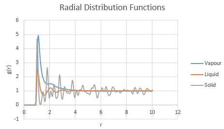
Unsurprisingly, the RDF is 0 for $r\le 0.9$. The Lennard-Jones repulsion term prevents the coexistense of atoms in this region below atomic diameter since such an overlap is physically impossible without great perturbation of the atomic structures (see Atomic Forces).

For the vapour phase, there is only one clear peak, with a possible secondary peak on its shoulder. This contrasts with the increasing number of peaks in the liquid and solid phases, as the system becomes more ordered and each particle experiences interactions with more neighbours at closer distances.

The liquid has a fairly smooth transition from

• peak one at ($r\approx 1$): a situation analagous to a solvation shell, with the First Nearest Neighbours included; $g(r)\approx 3.5$
• peak two at ($r\approx 2$): there are fewer Second Nearest Neighbours than First, in a similar way to how a primary solvation shell solvates tightly around a central ion, thus limiting the size of the outer hydration shell. Also for this peak, $g(r)\approx 1.25$, implying that molecules are half as likely to be found at this separation than at the separation defined by the first peak (since the $g(r)$ is half the size)
• peak three at ($r\approx 3$): the next nearest neighbours are suficiently far away to be tending towards bulk solution, with minimal attractive interaction

The first, second and subsequent troughs are the repulsions experienced between the central atom and opposing atoms and minimalise as the distance increases.

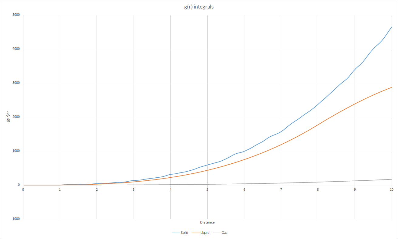
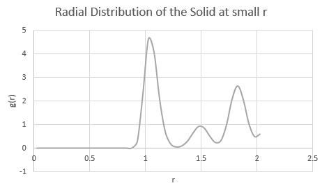
JC: If you zoom in on the integral of the solid RDF at small r you can see the jumps which correspond to the first 3 peaks and show directly the number of nearest neighbours responsible for each of the peaks.

The first three peaks of the RDF of the solid are seen to be more defined than for the liquid and vapour phases in which the atoms are not fixed in place and are more free to move. The atoms in a solid are fixed in position at given lattice points - and thus experience consistent interactions with neighbouring atoms.

Additionally, the amplitude of the peaks endure at higher levels and higher $r$ values in the RDF for the solid phase, implying that long range order permeates to longer distances in a solid than in the other phases. This is reasonable when the structure of a solid is considered relative to the disorder of gases and liquids.

Moreover, the lattice spacing may be deduced from the RDF of the solid by correlating the peak to points on the lattice. The first peak corresponds to the nearest neighbours to a given atom (of which there are 12 for an fcc lattice). The second peak corresponds to the lattice spacing which is therefore equivalent to $d\approx 1.49$ for this solid. The third peak, with $g(r_3)\approx \frac{1}{2}g(r_1)$ (i.e. g(r) = 2.4 at r = 1.825, which is roughly half of g(r) (=4.6) at 1.025, corresponds to the third nearest neighbour shell. The coordination numbers are 12 for the first shell, 6 for the second nearest shell and 24 for the third nearest shell.

JC: Good description of how the solid RDF relates to the structure of the solid phase, compared to the liquid and vapour RDFs.

Coordination number at distance $r_A=4\pi \int g(r)r^2\mathrm{d}r$

Mean Squared Displacement and the Diffusion Coefficient

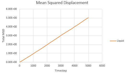
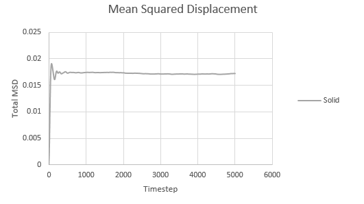
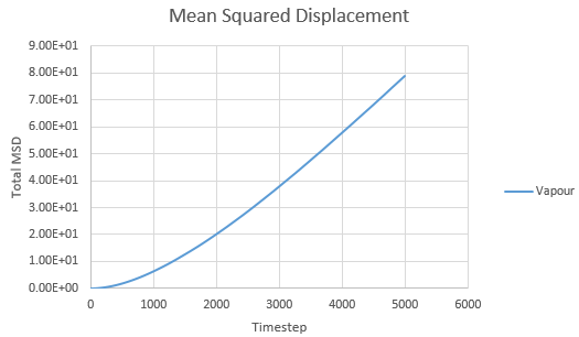
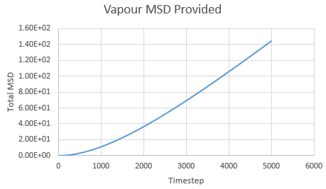
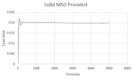
Mean squared displacement calculations model how variable the system is. Hence MSD for a solid < liq < vapour.

The values input for the calculations were as follows:

Vapour:

Reduced density = 0.05

Reduced Temperature = 0.75

Liquid:

Reduced density = 0.8

Reduced Temperature = 1.2

Solid:

Reduced density = 1.2

Reduced Temperature = 1.2

JC: It would have been good to have shown the linear fits to the MSDs on your plots.

Evaluation of the normalised velocity autocorrelation function for a 1D harmonic oscillator

The diffusion coefficient is calculated using the formula $D=\frac{1}{6}\frac{\partial ⟨r^2\left(t\right)⟩}{\partial t}$

And thus is simply $\frac{gradientoftheMSDcurves}{6}$ However, we must convert the value of the gradient from timesteps into time using the reduced units. Since the value of the timesteps was 0.002, the measured gradient is simply divided by 0.002 to give the diffusion coefficient in correct units.

Solid: Liquid: Gas:

State	Data	Gradient	D
Solid	Simulated	5 x 10-8	4.17 x 10-6
Solid	Provided	5 x 10-8	4.17 x 10-6
Liquid	Simulated	0.001	8.3 x 10-2
Liquid	Provided	0.001	8.3 x 10-2
Gas	Simulated	0.0167	1.39
Gas	Provided	0.0305	2.54

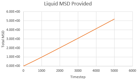
As expected, the MSD is largest for a gas and smallest for a solid in which the system remains relatively static. Moreover, the MSD equilibrates for a solid since the atoms and sit on fixed lattice points.

The simulated and provided data give concordant results to equivalent or very similar values for each phase. Therefore using a million atoms is not justified in terms of cost for the calculations of MSD.

Evaluation of the normalised velocity autocorrelation function for a 1D harmonic oscillator:

$C\left(\tau \right)=\frac{\underset{-\mathrm{\infty }}{\overset{\mathrm{\infty }}{\int }}v\left(t\right)v(t+\tau )\mathrm{d}t}{\underset{-\mathrm{\infty }}{\overset{\mathrm{\infty }}{\int }}{v}^2\left(t\right)\mathrm{d}t}$

The position of a 1D harmonic oscillator as a function of time is given by

$x\left(t\right)=A\cos (\omega t+\varphi )$

Considering that the velocity is defined by

$v\left(t\right)=\frac{\mathrm{d}x}{\mathrm{d}t}$

We can apply the chain rule to define $v\left(t\right)$ :

set $u$to equal $(\omega t+\varphi )$

$\frac{\mathrm{d}u}{\mathrm{d}t}=\omega$

hence

$\frac{\mathrm{d}}{\mathrm{d}t}A\cos (\omega t+\varphi )=A\cos \left(u\right)$

$=\frac{\mathrm{d}}{\mathrm{d}u}A\cos \left(u\right)\frac{\mathrm{d}u}{\mathrm{d}t}$

$=-A\sin \left(u\right)\omega$

$=-A\omega \sin (\omega t+\varphi )$

$=v$

For the velocity at time $t+\tau$ relative to time $t$ we adapt the equation for $v$:

$v(t+\tau )=\frac{\mathrm{d}x}{\mathrm{d}(t+\tau )}$

$=-A\omega \sin (\omega (t+\tau )+\varphi )$

$=-A\omega \sin (\omega t+\omega \tau )+\varphi )$

this may then be substituted into the autocorrelation function to give:

$C\left(\tau \right)=\frac{\underset{-\mathrm{\infty }}{\overset{\mathrm{\infty }}{\int }}v\left(t\right)v(t+\tau )\mathrm{d}t}{\underset{-\mathrm{\infty }}{\overset{\mathrm{\infty }}{\int }}{v}^2\left(t\right)\mathrm{d}t}$

$=C\left(\tau \right)=\frac{\underset{-\mathrm{\infty }}{\overset{\mathrm{\infty }}{\int }}-A\omega \sin (\omega t+\varphi )-A\omega \sin (\omega t+\omega \tau )+\varphi )\mathrm{d}t}{\underset{-\mathrm{\infty }}{\overset{\mathrm{\infty }}{\int }}-A^2{\omega }^2{\sin }^2(\omega t+\varphi )\mathrm{d}t}$

$=C\left(\tau \right)=\frac{\underset{-\mathrm{\infty }}{\overset{\mathrm{\infty }}{\int }}A\omega \sin (\omega t+\varphi )A\omega \sin (\omega t+\omega \tau )+\varphi )\mathrm{d}t}{\underset{-\mathrm{\infty }}{\overset{\mathrm{\infty }}{\int }}A\omega \sin (\omega t+\varphi )A\omega \sin (\omega t+\varphi )\mathrm{d}t}$

$=C\left(\tau \right)=\frac{\underset{-\mathrm{\infty }}{\overset{\mathrm{\infty }}{\int }}\sin (\omega t+\varphi )\sin (\omega t+\omega \tau )+\varphi )\mathrm{d}t}{\underset{-\mathrm{\infty }}{\overset{\mathrm{\infty }}{\int }}\sin (\omega t+\varphi )\sin (\omega t+\varphi )\mathrm{d}t}$

This may then be expanded using the trigonomic identity

$\sin (x+y)=\sin \left(x\right)\cos \left(y\right)+\cos \left(x\right)\sin \left(y\right)$

to give:

$C\left(\tau \right)=\frac{\underset{-\mathrm{\infty }}{\overset{\mathrm{\infty }}{\int }}\sin (\omega t+\varphi )[\sin \left(\omega \tau \right)\cos (\omega t+\varphi )+\cos \left(\omega \tau \right)\sin (\omega t+\varphi )\mathrm{d}t}{\underset{-\mathrm{\infty }}{\overset{\mathrm{\infty }}{\int }}{\sin }^2(\omega t+\varphi )\mathrm{d}t}$

$=\frac{\underset{-\mathrm{\infty }}{\overset{\mathrm{\infty }}{\int }}\sin (\omega t+\varphi )\sin \left(\omega \tau \right)\cos (\omega t+\varphi )+{\sin }^{}(\omega t+\varphi )\cos \left(\omega \tau \right)\mathrm{d}t}{\underset{-\mathrm{\infty }}{\overset{\mathrm{\infty }}{\int }}{\sin }^2(\omega t+\varphi )\mathrm{d}t}$

$=\frac{\underset{-\mathrm{\infty }}{\overset{\mathrm{\infty }}{\int }}\sin (\omega t+\varphi )\sin \left(\omega \tau \right)\cos (\omega t+\varphi )+\mathrm{d}t}{\underset{-\mathrm{\infty }}{\overset{\mathrm{\infty }}{\int }}{\sin }^2(\omega t+\varphi )\mathrm{d}t}+\frac{\underset{-\mathrm{\infty }}{\overset{\mathrm{\infty }}{\int }}{\sin }^2(\omega t+\varphi )\cos \left(\omega \tau \right)\mathrm{d}t}{\underset{-\mathrm{\infty }}{\overset{\mathrm{\infty }}{\int }}{\sin }^2(\omega t+\varphi )\mathrm{d}t}$

$=\frac{\sin \left(\omega \tau \right)\underset{-\mathrm{\infty }}{\overset{\mathrm{\infty }}{\int }}\sin (\omega t+\varphi )\cos (\omega t+\varphi )+\mathrm{d}t}{\underset{-\mathrm{\infty }}{\overset{\mathrm{\infty }}{\int }}{\sin }^2(\omega t+\varphi )\mathrm{d}t}+\frac{\cos \left(\omega \tau \right)\underset{-\mathrm{\infty }}{\overset{\mathrm{\infty }}{\int }}{\sin }^{}(\omega t+\varphi )\mathrm{d}t}{\underset{-\mathrm{\infty }}{\overset{\mathrm{\infty }}{\int }}{\sin }^2(\omega t+\varphi )\mathrm{d}t}$

$=\frac{\sin \left(\omega \tau \right)\underset{-\mathrm{\infty }}{\overset{\mathrm{\infty }}{\int }}\sin (\omega t+\varphi )\cos (\omega t+\varphi )+\mathrm{d}t}{\underset{-\mathrm{\infty }}{\overset{\mathrm{\infty }}{\int }}{\sin }^2(\omega t+\varphi )\mathrm{d}t}+\cos \left(\omega \tau \right)$

Thence, the first term $=\frac{\sin \left(\omega \tau \right)\underset{-\mathrm{\infty }}{\overset{\mathrm{\infty }}{\int }}\sin (\omega t+\varphi )\cos (\omega t+\varphi )+\mathrm{d}t}{\underset{-\mathrm{\infty }}{\overset{\mathrm{\infty }}{\int }}{\sin }^2(\omega t+\varphi )\mathrm{d}t}$

simplifies to zero using the identity

$\underset{-\mathrm{\infty }}{\overset{\mathrm{\infty }}{\int }}\sin \left(x\right)\cos \left(x\right)\mathrm{d}t=0$

Hence

$C\left(\tau \right)=\cos \left(\omega \tau \right)$

JC: Final answer is correct, but some of your derivation is not very clear.

Velocity Autocorrelation Function

Above VACF versus time graphs plotted using the data provided

Above VACF versus time graphs plotted using own data, to a time of 500

The minima in the VACF plots are due to collisions occurring between atoms in the system. When two atoms collide, their directions are altered. However, the liquid (Figures 22 and 25) returns to a $VACF=0$ more rapidly than a solid (Figures 23 and 26) since there is less structure in a liquid compared to the denser, more rigid solid structure. Conversely, the harmonic oscillator is modeled as two atoms on a spring, hence the VASF simply oscillates periodically about $VACF=0$ .

JC: Did you manage to plot the running averages for the VACFs or calculate the diffusion coefficients?