Talk:Mod:AB9197

JC: General comments: Well written report with clear, detailed explanations which show a good understanding of the underlying theory behind the experiment. Good use of extra analysis and material to enhance explanations, but make sure that you fully answer all of the questions.

Simulation of a Simple Liquid - Year 3 Computational Lab

The Simplest Case - Simulation of a Harmonic Oscillator

The position $x$ of a harmonic oscilllator with angular frequency $\omega$, amplitude $A$ and phase shift $\varphi$ is given by $x=A\cos (\omega t+\varphi )$. This position was compared against the position $x_{vv}$ obtained from the velocity-Verlet algorithm by plotting the absolute error $|x-x_{vv}|$ against $t$ as shown in Figure 1. Throughout this analysis, the values of the parameters were $\omega =A=1$ and $\varphi =0$ with a value of the timestep of 0.1.

Figure 1: Absolute error in position of harmonic oscillator as calculated by the velocity-verlet algorithm against the exact analytical solution

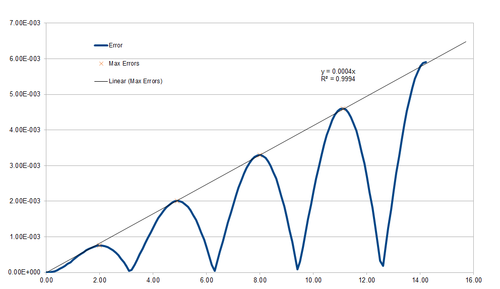
Clearly, the error undergoes oscillations with period $\pi$, while the magnitude of the oscillations increases linearly in time, with $\mathrm{E}\mathrm{r}\mathrm{r}\mathrm{o}\mathrm{r}=0.0004t$. Intuitively, this makes sense, as we expect the error to accumulate over time.

JC: Why does the error oscillate over time?

Another important measure of the success of the simulation is the variation of the total energy in time. Since the harmonic oscillator is considered as an isolated system, we expect this to remain constant in time. In fact, the sum of the potential and kinetic energies, as calculated from the simulated positions and velocities, was also found to oscillate with period $\pi$. However the magnitude of these oscillations constituted only 1% of the total energy even at a timestep value of 0.28. Thus we may say that energy is conserved to a close approximation - especially when considered over a larger timeframe - in our simulation, and that therefore the velocity-Verlet algorithm has performed well.

Some Practical Aspects of Simulations

Atomic Forces - The Lennard-Jones Potential

The potential energy of interaction between any two particles in the simulations is approximated by the Lennard-Jones potential:

$\varphi (r)=4ϵ(\frac{{\sigma }^{12}}{r^{12}}-\frac{{\sigma }^6}{r^6})$

Where $r$ is the interparticle centre-centre separation. This evaluates to zero at $r=r_0=\sigma$.

Since the force experienced by a particle in a potential $U(r)$ is given by $F(r)=-\frac{dU}{dr}$, the force at $r_0$ is found by evaluating the derivative of the Lennard-Jones potential with respect to $r$ at $r=\sigma$, giving $F(r)=24ϵ(2\frac{{\sigma }^{12}}{r^{13}}-\frac{{\sigma }^6}{r^7})$, and thus $F(\sigma )=\frac{24ϵ}{\sigma }$.

Two interacting particles are said to be at equilibrium if there are no forces acting on either particle. If their interaction is well-described by a Lennard-Jones potential, solving $F(r)=0$ yields $r_{eq}=2^{\frac{1}{6}}\sigma$. At this separation, the depth of the potential is $\varphi (r_{eq})=-ϵ$.

When implementing the Lennard-Jones potential, the computational expense is significantly reduced by introducing a cut-off inter-particle separation, beyond which the interaction potential is set to zero. To show that this may be chosen in such a way as to not significantly affect the validity of the simulation, we evaluate the following integrals, taking $ϵ=\sigma =1$ for simplicity:

$I_1=\underset{2\sigma }{\overset{\mathrm{\infty }}{\int }}\varphi (r)dr{I}_2=\underset{2.5\sigma }{\overset{\mathrm{\infty }}{\int }}\varphi (r)dr{I}_3=\underset{3\sigma }{\overset{\mathrm{\infty }}{\int }}\varphi (r)dr$

Thus, $I_1=4[\frac{1}{5r^5}-\frac{1}{11r^{11}}{]}_{2\sigma }^{\mathrm{\infty }}=-0.0248$, and similarly, $I_2=-0.0082$ and $I_3=-0.0033$. This illustrates how quickly the Lennard-Jones potential converges to zero as $r$ increases, since the area between the potential curve and the x-axis for $3\sigma ⩽r⩽\mathrm{\infty }$ is only about 15% of that for $2\sigma ⩽r⩽2.5\sigma$. These values appear dimensionless only because we have taken $ϵ=\sigma =1$, i.e. are working in Lennard-Jones units, but really, they have units of energy*distance. Also, $\frac{\varphi (3\sigma )}{\varphi (r_{eq})}=0.005$, i.e. the interaction energy of two particles with centre-to-centre separation $3\sigma$ is only 0.5% of that of two particles separated by $r_{eq}=2^{\frac{1}{6}}\sigma$.

JC: All maths correct and integrals well explained.

Approximating Bulk - Periodic Boundary Conditions

$1\text{<mrow data-mjx-texclass="ORD">mL</mrow>}$ of water has a mass of roughly 1 g, and thus contains approximately $3.34\times 10^{22}$ molecules. 10000 water molecules occupy a volume of $2.99\times 10^{-19}\text{<mrow data-mjx-texclass="ORD">mL</mrow>}$. Since simulating on the order of $10^{22}$ molecules is an unrealistic proposition, some way of investigating the bulk properties from smaller simulations must be used. An elegant solution is to implement periodic boundary conditions, meaning that, when a particle is predicted to leave the simulation box, it instead re-enters the simulation box in the same way as it would if entering from an adjacent box, if the box were placed in an infinite lattice. As an example, let us consider a cubic box with side lengths 1, placed in such a way that one vertex lies on the origin and another at $(1,1,1)$. An atom with initial position $(0.5,0.5,0.5)$ is changing its position by $(0.7,0.6,0.2)$ every timestep. When periodic boundary conditions are applied, after a single timestep it will be found at $(0.2,0.1,0.7)$.

JC: Values are correct, but would be good to show some working.

Keeping it Simple - Reduced Units

In order to avoid having to handle exceedingly large or small numbers, simulations are often performed with dimensionless reduced units. Additionally, this allows the output of the simulation to be used to represent different physical systems, simply by choosing the appropriate conversion factors. Of course, to obtain accurate values, the simulation must still provide a realistic model of all systems considered. In this investigation, so-called Lennard-Jones (LJ) units were used, and output values converted to SI units for the case of pure Argon. The appropriate equations are:

distance $r^{*}=\frac{r}{\sigma }$

energy $E^{*}=\frac{E}{ϵ}$

time $t^{*}=t\frac{{ϵ}^{\frac{1}{2}}}{m^{\frac{1}{2}}\sigma }$

temperature $T^{*}=\frac{k_{B}T}{ϵ}$ For Argon, $\sigma =3.4\times 10^{-10}\text{m}$, $ϵ=1.66\times 10^{-21}\text{J}$ and $m=6.69\times 10^{-26}\text{<mrow data-mjx-texclass="ORD">kg</mrow>}$. Thus, a reduced temperature of $T^{*}=1.5$ corresponds to an actual temperature of $T=180\text{K}$, $r^{*}=3.2\equiv r=1.1\text{<mrow data-mjx-texclass="ORD">nm</mrow>}$ and the LJ potential well depth is $-ϵ=-1.66\times 10^{-21}\text{J}=-0.998\text{<mrow data-mjx-texclass="ORD">kJ<mo lspace="0" rspace="0">/</mo>mol</mrow>}$.

JC: Correct.

Creating the Simulation Box

When initialising our simulation box, the coordinates of the particles are not assigned randomly, since doing so could result in some particles being significantly more closely spaced than the LJ equilibrium separation. Two particles in such a situation would possess a very high potential energy and experience huge forces, and would thus fly apart with great kinetic energies, increasing the temperature of the simulation and perhaps obscuring otherwise interesting phenomena.

JC: High repulsive forces can cause the simulation to become unstable and crash.

The number density of lattice points for a simple cubic lattice is simply $\frac{1}{L^3}$, where $L$ is the side length of the unit cell, and thus also the closest distance between two lattice points. Thus, if the number density is 0.8, $L=(\frac{1}{0.8}{)}^{\frac{1}{3}}=1.07722$. A face-centred cubic lattice contains four lattice points per unit cell, and so the lattice point density is given by $\frac{4}{L^3}$. Therefore, for a lattice point density of 1.2, $L=(\frac{4}{1.2}{)}^{\frac{1}{3}}=1.4938$.

If a 10x10x10 box of such simple cubic unit cells is created, and identical atoms placed at all lattice points, the result is a 10.7722x10.7722x10.7722 regular array containing 1000 atoms. If, on the other hand, a face-centred cubic cell as defined above was used, the array would instead measure 14.938x14.938x14.938, and contain 4000 atoms, since each fcc unit cell contributes four lattice points.

JC: Correct.

Setting the Properties of the Atoms

Consider the following piece of code:

mass 1 1.0
pair_style lj/cut 3.0
pair_coeff * * 1.0 1.0

The first line sets the mass of all atoms of type 1 (in this case, all atoms are of type 1) to 1.0 (in reduced units). The pair_style command in the second line sets the formula used to compute pairwise interactions. In this case, the style lj/cut means that a Lennard-Jones potential is used, with all pairwise interactions with centre-centre separation greater than 3 discarded. The last line contains the pair_coeff command, which sets the interaction coefficients of a particular pair of atom types in accordance with the specified pair_style (the LJ potential). In this case, the two asterisks indicate that any combination of atom pairs interact according to the LJ potential with $ϵ=\sigma =1.0$.

Since the initial positions of the atoms have been set to coincide with the lattice points of a simple cubic lattice, and the initial velocities can be expected to follow the Maxwell-Boltzmann distribution, it is the velocity-Verlet algorithm that performs the simulations.

JC: Correct.

Running the Simulation

In all input files, the length of each timestep (in reduced units) is defined as the 'timestep' variable and used to compute the number of timesteps required to reach $T^{*}=100$. This ensures that the length of time simulated is always the same, since only then can the output from simulations using different timesteps be compared.

Figure 3: Top left: Plot of pressure against time for timestep = 0.001; Top right: Temperature against time for timestep = 0.001; Bottom left: Energy against time for timestep = 0.001; Bottom right: Energy against time for different timesteps

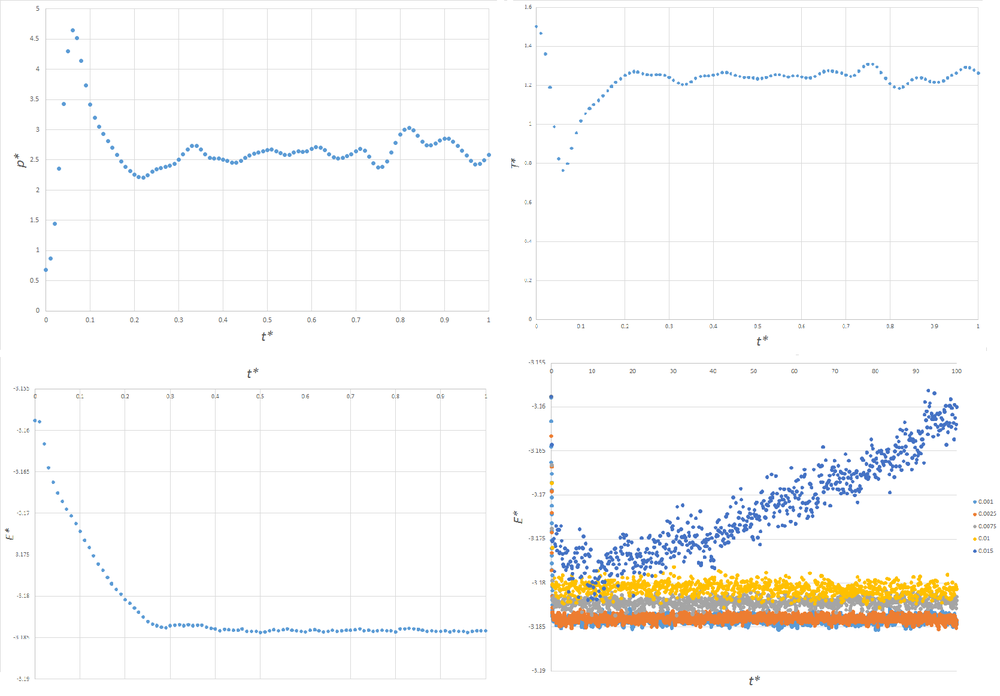
Figure 3 shows plots of the energy, pressure and temperature of simulations for a timestep of 0.001, and a plot of the total energies of simulations using a variety of timesteps. Clearly, for a timestep of 0.001, the system has reached equilibrium by $t*=0.3$, as pressure, temperature and energy are fluctuating around converged values. It can be seen that when the timestep = 0.015, the energy does not converge. As the size of the timesteps decreases, the total energy converges to a more negative value, and the magnitude of random fluctuations in the energy decrease. This matches our intuition, since the simulation is expected to more closely match the real behaviour of the system at smaller timesteps, and the real behaviour expected to lead to lower energies than an approximate algorithm. Thus, a timestep of 0.015 is too large to produce meaningful results. The best compromise between accuracy and computational expense is therefore a timestep of 0.0025, since the random fluctuations in energy overlap with the slightly lower energy to which the simulation with a timestep of 0.0025 converges.

JC: Good choice of timestep, but why did you not choose 0.01 or 0.0075, should the average total energy should not depend on the timestep? Why is it better to set the timestep using a variable?

Running Simulations Under Specific Conditions

Controlling the Temperature

Often, it is required that the the temperature is constant. By the equipartition theorem, each accessible degree of freedom of our system receives $\frac{1}{2}{k}_{B}T$ of thermal energy , and so, for a 3-dimensional monoatomic system, the total kinetic energy is $E_K=\frac{1}{2}\sum _j{m}_j{v}_j^2=\frac{3}{2}{k}_{B}T$. If this instantaneous temperature is calculated at every timestep, fluctuations are found to occur.. To counteract these, the velocities of all particles are scaled by a factor $\gamma$ in such a way as to achieve the target temperature $\mathfrak{𝔗}$. Thus:

$\frac{1}{2}\sum _j{m}_j{v}_j^2=\frac{3}{2}{k}_{B}T$

$\frac{1}{2}\sum _j{m}_j(\gamma v_j{)}^2=\frac{3}{2}{k}_B\mathfrak{𝔗}$.

Which, upon division, yields

$\gamma =\sqrt{\frac{\mathfrak{𝔗}}{T}}$

JC: Good derivation.

Recording Data Points

A variety of simulations were performed in the NpT ensemble, that is, with the number of particles, pressure and temperature all kept constant. The timestep was chosen to be $0.0025t^{*}$. A quantity of interest was the average density of the system, and so below is the part of the input file responsible for recording the averages of various quantities:

### MEASURE SYSTEM STATE ###
thermo_style custom step etotal temp press density
variable dens equal density
variable dens2 equal density*density
variable temp equal temp
variable temp2 equal temp*temp
variable press equal press
variable press2 equal press*press
fix aves all ave/time 100 1000 100000 v_dens v_temp v_press v_dens2 v_temp2 v_press2
run 100000

The three numbers '100 1000 100000' mean that every 100000 timesteps, the average values of all of the following variables, as computed 1000 times every 100 timesteps previously, are calculated. Since each simulation is run over 100000 timesteps (at timestep = 0.01, $1000t^{*}\equiv 2.17\times 10^{-9}s$, for Argon), the averages are only calculated once at the end.

Plotting Equations of State

Figure 4: Density at different densities for simulation and ideal gas

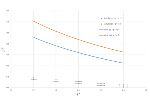
Figure 4 shows a plot of density against temperature, both for simulations (in the NpT ensemble), and as given by the ideal gas law. Note that the y-errorbars are not visible on the scale of this graph. Clearly, the densities predicted by the ideal gas law are much larger than those obtained from the simulations. This is a result of the fact that the ideal gas law does not take any form of atom-atom interactions into account, and is thus much more compressible than the simulated LJ-liquid simulated, where interactions rapidly become unfavourable at small spacings. More explicitly, if the LJ-liquid were present - initially in a simple cubic lattice - at the density predicted by the ideal gas law at $T^{*}=1.7$ and $P^{*}=2.5$, namely ${\rho }^{*}=1.47$, the nearest-neighbour separation would be $\frac{1}{1.47^{\frac{1}{3}}}=0.315$ and so significantly shorter than $r_{eq}=1.122$. On average, any two nearest-neighbours would thus feel large repulsive forces, and so clearly this does not present a stable system. At the higher pressure, the discrepancy between the simulation and the ideal gas law is even larger, as the average atomic spacing will be smaller, and thus the repulsive forces arising from the LJ potential larger, even more remote from the ideal-gas description of matter.

Both for the ideal gas and the simulated system, the density decreases with temperature, as may be expected, since an NpT system expands such as to keep the pressure constant as the temperature increases.

JC: Very good explanation nicely illustrated with nearest neighbour distance calculation.

Calculating the Heat Capacity

In the canonical ensemble, where the number of particles, occupied volume and temperature are fixed, the constant-volume heat capacity is given by $C_V=\frac{\partial E}{\partial T}=\frac{Var[E]}{k_B{T}^2}$. To observe the variation of the heat capacity with temperature and pressure, simulations were run at pressures of $P^{*}=0.2$ and $P^{*}=0.8$ and temperatures of $T^{*}=2.0;2.2;2.4;2.6;2.8$ at each pressure. To compare the output values (in reduced units) to literature, it is necessary to multiply by the relevant conversion factors, giving $C_V=\frac{Var[E^{*}]}{{T^{*}}^2}$. However, since heat capacity is an extensive property, it is more insightful to study the behaviour of $\frac{C_V}{V}=\frac{C_V}{{\sigma }^3{V}^{*}}$.

Results

Figure 5: Volumetric constant-volume heat capacity as a function of temperature, at reduced densities 0.2 and 0.8

Figure 6: Comparison between molar constant-volume heat capacities as a function of temperature at reduced densities 0.2 and 0.8, as obtained through MD simulations and literature values from the NIST.

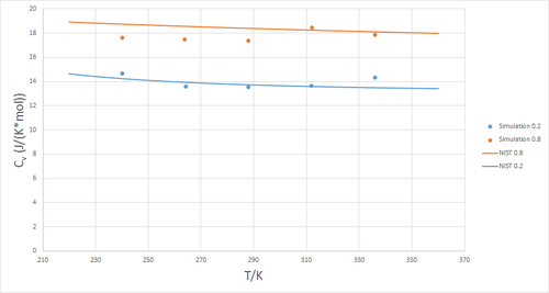
Figure 5 shows a plot of the volumentric heat capacity at constant volume as a function of temperature, evaluated at two different pressures ${\rho }^{*}=0.2\equiv \rho =340.4\mathrm{k}\mathrm{g}{\mathrm{m}}^{\mathrm{-}\mathrm{3}}$ and ${\rho }^{*}=0.8\equiv \rho =1361.7\mathrm{k}\mathrm{g}{\mathrm{m}}^{\mathrm{-}\mathrm{3}}$. Commonly, heat capacity increases with temperature as more degrees of freedom, such as rotational and vibrational modes, are able to 'store' thermal energy. Clearly, this is not the case here, which can be attributed to the absence of any such additional degrees of freedom in a monoatomic fluid. To verify this data, it was compared to that of the National Institute of Standards and Technology (NIST). As can be seen in figure 6, the data obtained from simulation provides a good match to that of the NIST.

An example of one of the input scripts is found here.

JC: Good idea to compare your data to other published data, but you should include more details about the NIST data, is this also for a monoatomic fluid, what temperature/pressure is it at? What about the trend with density?

The Radial Distribution Function

A convenient measure of the spatial arrangements of atoms is the radial distribution function (RDF) $g(r)$. It represents a measure of the variation in the density relative to the bulk average density, and so $\rho (r)={\rho }_{avg}g(r)$.

The RDF in Different Phases

Intuitively, the more ordered phases can be expected to show greater variation in the RDF, since, in a perfect crystal, it would peak sharply at separations corresponding to lattice points, and be zero otherwise. In the presence of disorder, $g(r)$ will converge to unity more ore less rapidly with distance, since the influence of local interactions on the structure will be masked by random thermal motion, and thus the density given by the average bulk density. At lower densities, where the average particle separation is larger and thus interactions less significant, and at higher temperatures, where thermal motion plays a greater role, the RDF will therefore be more likely to decay in a simple manner. As the density (generally) decreases and the temperature increases in going from a solid to liquid to gaseous phase, these trends are borne out in figure 7, showing the RDF for each of the three phases:

Figure 7: Radial distribution function as a function of r* for solid, liquid and gas.

Figure 8: Integral of radial distribution function against r* for solid

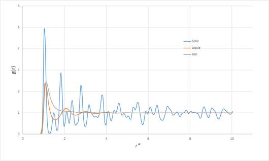
Particularly interesting is the RDF of the solid. When the trajectory of the simulation is viewed, the motion corresponds simply to vibrations of the face-centred cubic (fcc) lattice. The first few peaks can thus unambiguously be assigned to the distances corresponding to the closest neighbours of any lattice point. Letting $L$ be the side length of the unit cell, some simple geometry shows the first three closest neighbours to occur at distances of $\frac{L}{\sqrt{2}}$, $L$ and $\frac{\sqrt{3}}{\sqrt{2}}L$. Since the density of the solid (for the case of Argon) was ${\rho }^{*}=1.2\equiv \rho =2043\mathrm{k}\mathrm{g}{\mathrm{m}}^{\mathrm{-}\mathrm{3}}$, which must also satisfy $\rho =\frac{4\times 6.69\times 10^{-26}}{L^3}$, we can deduce that $L=5.08\times 10^{-10}\mathrm{m}$. From the RDF, the first peak occurs at $r^{*}=1.025\equiv r=3.49\times 10^{-10}\mathrm{m}$, the second at $r^{*}=1.475\equiv r=5.02\times 10^{-10}\mathrm{m}$ and the third at $r^{*}=1.825\equiv r=6.21\times 10^{-10}\mathrm{m}$. The three closest-neighbour separations of a perfect fcc lattice with the same density would be $3.59\times 10^{-10}\mathrm{m}$, $5.08\times 10^{-10}\mathrm{m}$ and $6.22\times 10^{-10}\mathrm{m}$. Clearly, these values are a good match.

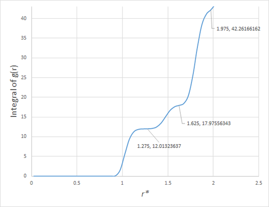
The coordination number of each of these peaks can be deduced from $\underset{0}{\overset{r}{\int }}g(r)$, and be compared to the number of lattice sites a distance $r$ from each lattice site in a perfect fcc lattice. In order of increasing separation, these are 12, 6 and 24.

As can be seen in figure 8, the area under the first peak in the RDF of the solid is 12, that under the second 6, and that under the third 24. Once again, the expected values of a fcc lattice match those obtained from the simulation very closely, and thus we can conclude that the simulated solid is indeed well-described as a fcc lattice. The LJ parameters necessary to obtain solid, liquid and gaseous phases were taken from Hansen and Verlet.

JC: Good analysis of the peaks in the solid RDF, a diagram of an fcc lattice with the first, second and third nearest neighbours marked would have been good. What about shape of the liquid and gas RDFs? The liquid RDF shows short range order, but no long range order.

Dynamical Properties and the Diffusion Coefficient

Figure 9: MSD against reduced time for a solid: small-scale simulation

Figure 10: MSD against reduced time for a solid: large-scale simulation

Figure 11: MSD against reduced time for a liquid: small-scale simulation

Figure 12: MSD against reduced time for a liquid: large-scale simulation

Figure 13: MSD against reduced time for a gas: small-scale simulation

Figure 14: MSD against reduced time for a gas: large-scale simulation

Estimating the Diffusion Coefficient Through the Mean Squared Displacement

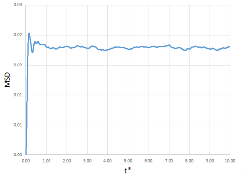
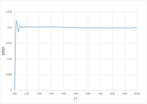
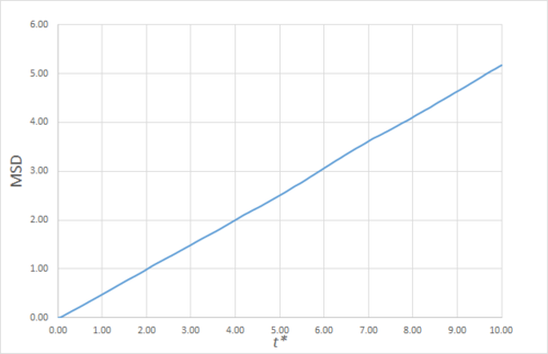
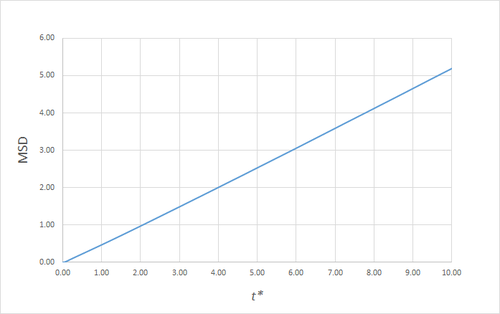
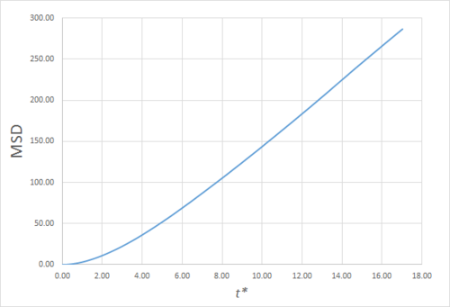
The mean squared displacement (MSD) is, as the name suggests, the mean of the square of the displacement of a given atom from its position at $t_0=0$ at a given time $t$. Its variation in time gives insight into the dynamical behaviour of the system under consideration. Thus, on the left and right are shown graphs of the MSD for solid, liquid and gaseous phases, with both around 10000 and around 1 million atoms simulated.

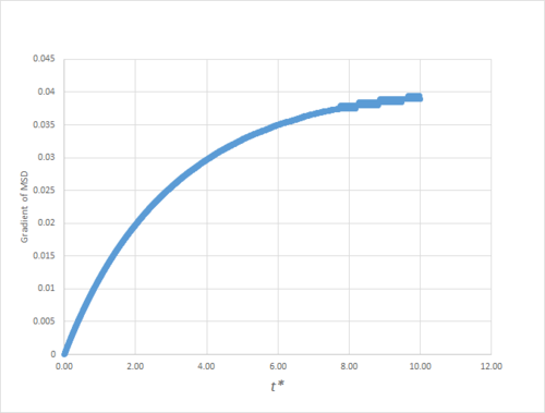
As can be seen in figures 9 to 14, the MSD converges to a straight line in most cases. The sole exception is the MSD of the large-scale gas simulation for which the data was provided, which had not fully approached a linear region. This was found by plotting the numerical gradient as a function of $t^{*}$. Thus, a smaller (~8000 atoms) simulation at the same conditions was run for 100000 timesteps, within which it did converge to a linear function. Clearly, the only differences between the two simulation sizes for each phase is the smoothness of the graph, with a larger simulation box resulting in a smoother MSD.

The self-diffusion coefficients were obtained by plotting the numerical derivatives and averaging the converged values, giving, in ${\mathrm{m}}^{\mathrm{2}}{\mathrm{s}}^{\mathrm{-}\mathrm{1}}$:

	Small Simulation	Large Simulation
Solid	$0$	$0$
Liquid	$4.62\times 10^{-9}$	$4.76\times 10^{-9}$
Gas	$1.83\times 10^{-7}$	$1.78\times 10^{-7}$*

The gradient of the MSD from which this value of the diffusion coefficient was obtained was not fully converged, as shown in figure 15,nand thus almost certainly underestimates the true value.

Figure 15: Gradient of MSD against reduced time for a gas: large-scale simulation

JC: It would have been good to plot the line of best fit on these graphs.

Estimating the Diffusion Coefficient Through the Velocity Auto-Correlation Function

The velocity autocorrelation function (VACF) is defined as $C(\tau )=⟨\overrightarrow{v}(t)\cdot \overrightarrow{v}(t+\tau )⟩$, in other words, it is the average of the inner products of the velocities at time $\tau$ with those at time $t$ averaged over all particles. In any system with random thermal motion, we therefore expect $\underset{\tau \to \mathrm{\infty }}{\lim }C(\tau )=0$, since each particle will be equally likely to be moving in any direction relative to its initial velocity, and thus $C(\tau )$ will average to zero.

Since, as in section 1.1, the position of a harmonic oscillator is given by $x(t)=A\cos (\omega t+\varphi )$, differentiation with respect to time gives the velocity as $v(t)=-\omega A\sin (\omega t+\varphi )$. Thus the velocity autocorrelation function (VACF)of a harmonic oscillator is:

$C(\tau )=\frac{\underset{-\mathrm{\infty }}{\overset{\mathrm{\infty }}{\int }}v(t)v(t+\tau )dt}{\underset{-\mathrm{\infty }}{\overset{\mathrm{\infty }}{\int }}v(t{)}^{2}dt}=\frac{{\omega }^2{A}^2\underset{-\mathrm{\infty }}{\overset{\mathrm{\infty }}{\int }}\sin (\omega t+\varphi )\sin (\omega t+\omega \tau +\varphi )dt}{{\omega }^2{A}^2\underset{-\mathrm{\infty }}{\overset{\mathrm{\infty }}{\int }}{\sin }^2(\omega t+\varphi )dt}$

Which, using the well-known double angle formula, can be written as:

$C(\tau )=\frac{\underset{-\mathrm{\infty }}{\overset{\mathrm{\infty }}{\int }}\sin (\omega t+\varphi )(\sin (\omega t+\varphi )\cos (\omega \tau )+\cos (\omega t+\varphi )\sin (\omega \tau ))dt}{\underset{-\mathrm{\infty }}{\overset{\mathrm{\infty }}{\int }}{\sin }^2(\omega t+\varphi )dt}=\frac{\cos (\omega \tau )\underset{-\mathrm{\infty }}{\overset{\mathrm{\infty }}{\int }}{\sin }^{}(\omega t+\varphi )dt+\sin (\omega \tau )\underset{-\mathrm{\infty }}{\overset{\mathrm{\infty }}{\int }}\sin (\omega t+\varphi )\cos (\omega t+\varphi )dt}{\underset{-\mathrm{\infty }}{\overset{\mathrm{\infty }}{\int }}{\sin }^2(\omega t+\varphi )dt}$

Substituting a new variable $u=\omega t+\varphi ⟹\frac{du}{dt}=\omega ⟹dt=\frac{du}{\omega }$ enables the second integral in the numerator to be written as the product of an even and an odd function of $u$, whilst the limits remain unchanged in the limit of $-\mathrm{\infty }$ and $\mathrm{\infty }$:

$C(\tau )=\frac{\cos (\omega \tau )\underset{-\mathrm{\infty }}{\overset{\mathrm{\infty }}{\int }}{\sin }^{}(u)du+\sin (\omega \tau )\underset{-\mathrm{\infty }}{\overset{\mathrm{\infty }}{\int }}\sin (u)\cos (u)du}{\underset{-\mathrm{\infty }}{\overset{\mathrm{\infty }}{\int }}{\sin }^2(u)du}$

Since the product of an even and an odd function is an odd function, and the integral of an odd function over a symmetric interval is zero, this simplifies to:

$C(\tau )=\frac{\cos (\omega \tau )\underset{-\mathrm{\infty }}{\overset{\mathrm{\infty }}{\int }}{\sin }^{}(u)du}{\underset{-\mathrm{\infty }}{\overset{\mathrm{\infty }}{\int }}{\sin }^2(u)du}=\cos (\omega \tau )$

JC: Well explained derivation.

The VACFs of the solid, liquid, and gas simulations, together with that of the harmonic oscillator for $\omega =\frac{1}{2\pi }$, $\cos (\omega \tau )$, are given in figure 16.

Figure 16: VACF of harmonic oscillator and solid and liquid simulations.

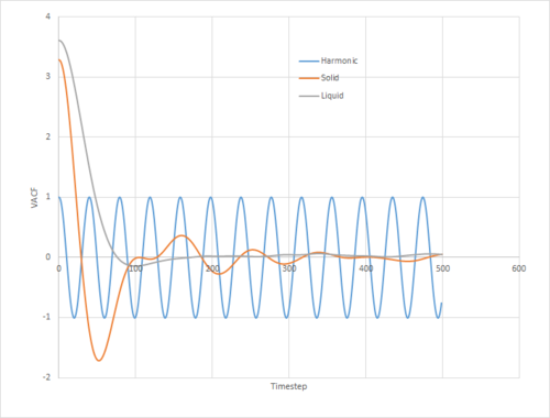
It can be seen that the VACF of the solid presents somewhat of an intermediate between that of the liquid simulation and the harmonic oscillator. On one extreme, the velocity of the harmonic oscillator follows a simple sinusoidal function. Clearly, since the velocity is an analytic function of time, at no point does it decorrelate from the original velocity. On the other hand, that of the liquid only displays one clear stationary point whilst rapidly decaying. Clearly then, there is a balance between ordered oscillatory motion due to collisions with the nearest neighbours, and exponential decorrelation due to random thermal motion and off-angle collisions. The former plays a more significant role in the movement of atoms in the solid, where they are strongly confined to their lattice sites, whilst the latter predominates that of the liquid.

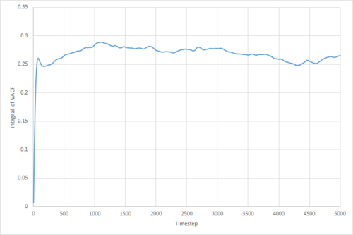
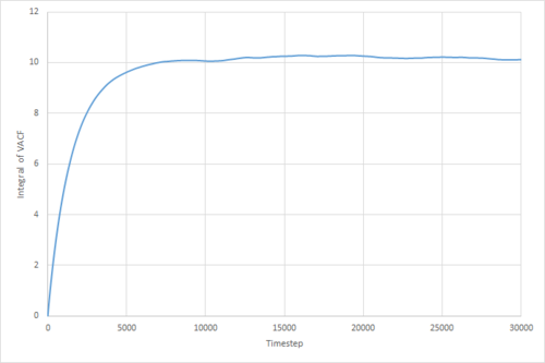
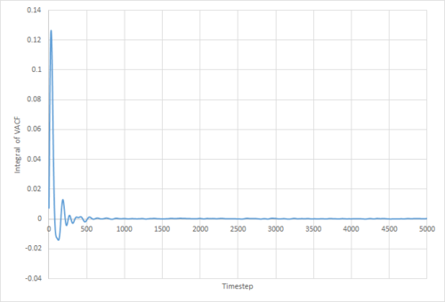
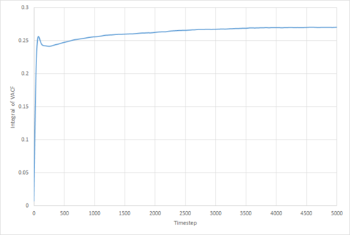
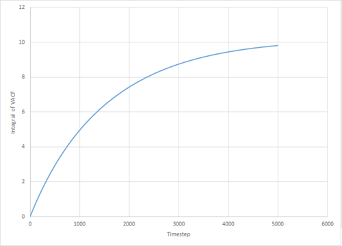
The VACF may be used to estimate the diffusion coefficient through the relation $D=\frac{1}{3}\underset{0}{\overset{\mathrm{\infty }}{\int }}⟨\overrightarrow{v}(0)\cdot \overrightarrow{v}(\tau )⟩d\tau$, assuming that the VACF converges to zero. To show that this is the case, and to evaluate the diffusion coefficients, the VACF was integrated using the trapezium rule. The resulting graphs of the cumulative integral as a function of the timestep for each of the three phases, and both the small- and large-scale simulations, are shown in figures 17 to 22.

Figure 17: MSD against reduced time for a solid: small-scale simulation	Figure 18: MSD against reduced time for a solid: small-scale simulation	Figure 19: MSD against reduced time for a solid: small-scale simulation
Figure 20: MSD against reduced time for a solid: small-scale simulation	Figure 21: MSD against reduced time for a solid: small-scale simulation	Figure 22: MSD against reduced time for a solid: small-scale simulation

Of note is the fact that the cumulative integral of the VACF for the solid simulation converges to zero. This implies that each atom moves in the direction opposite to its original velocity for the same distance as it does in parallel to it in the limit of large timescales, and thus overall is not displaced significantly. This is consistent with the idea that in a solid fcc lattice, the atoms are localised at their respective lattice sites, only vibrating over small distances.

Once again, the provided data for the large-scale gas simulation had not converged, and so the small-scale simulation was run to a larger number of timesteps. The resulting diffusion coefficients, converted to units of ${\mathrm{m}}^{\mathrm{2}}{\mathrm{s}}^{\mathrm{-}\mathrm{1}}$ using the LJ parameters for Argon, are thus:

	Small Simulation	Large Simulation
Solid	$0$	$0$
Liquid	$4.81\times 10^{-9}$	$4.81\times 10^{-9}$
Gas	$1.82\times 10^{-7}$	$1.75\times 10^{-7}$

Which are all within 5% of the values obtained through use of the MSD method. The two largest sources of error in these values are likely to be statistical inaccuracies due to insufficient ensemble size and length of the simulation. Clearly, the variance in the 'converged' VACF integral is much larger for the smaller simulations, and it has been shown by Zwanzig and Aliwadi that the statistical error in the VACF varies with $\frac{1}{n^{\frac{1}{2}}}$ and with $\frac{1}{t^{\frac{1}{2}}}$ , where $n$ is the ensemble size and $t$ the time length of the simulation. Of course, since both the MSD and integrated VACF of the large-scale gas simulation provided had not converged to their respective linear/constant limits, the thusly obtained values underestimate the true value.

The error in the values obtained through the MSD are likely to arise mainly from the effects of the initial conditions. Pranami and Lamm showed that the time taken for the ergodic hypothesis to apply - in other words, after what time the time average of a property is equal to the ensemble average - can be significantly larger than the timescales typically employed in MD simulations of LJ fluids. Their proposed improvement was to instead perform many independent shorter simulations such as to reduce the otherwise resulting errors.

JC: Nice analysis and use of extra material from the literature.

References

- ↑ D. Chandler, Introduction to Modern Statistical Mechanics, Oxford University Press, New York, 1987.
- ↑ E.W. Lemmon, M.O. McLinden and D.G. Friend, "Thermophysical Properties of Fluid Systems" in NIST Chemistry WebBook, NIST Standard Reference Database Number 69, Eds. P.J. Linstrom and W.G. Mallard, National Institute of Standards and Technology, Gaithersburg MD, 20899, http://webbook.nist.gov, (retrieved October 20, 2016).
- ↑ J.-P. Hansen and L. Verlet, Phys. Rev., 1969, 184, 151–161.
- ↑ R. Zwanzig and N. K. Ailawadi, Phys. Rev., 1969, 182, 280–283.
- ↑ G. Pranami and M. H. Lamm, J. Chem. Theory Comput., 2015, 11, 4586–4592.