Talk:Mod:636752
JC: General comments: All tasks answered with a few mistakes and report nicely laid out. Include a bit more detail in some of your explanations and analysis to show that you understand what your data is telling you and why you observe the trends that you do.
Task 1: Lowest energy state
The energy minimum corresponds to the configuration having all the spins aligned (either si=1 or si=-1 for any i between 1 and N). Therefore, si sj=1 for either of these possibilities, so the energy becomes:
In order to evaluate the inner sum we have to figure out how many neighbours each spin has. It can be easily noticed that for a D-dimensional lattice each spin has 2D neighbours.
For the minimum energy macrostate there are two possible microstates: either when all spins are 1, or when all spins are -11. Therefore, the multiplicity of this macrostate is . This is related to entropy by Boltzmann’s equation: . In this case:
Task 2: Flip one spin
If we take the the configuration with all spins aligned and flip one the only changing interactions are those between the spin we flip and its neighbours. Again, for a D-dimensional lattice there are 2D neighbours for each spin. Therefore, when the spin is flipped, the energy of every interaction (between the chosen spin and its neighbours) changes from –J to J, so there is a change in energy of 2J per interaction. Considering there is an interaction with every neighbour, the total change in energy will be
For D=3 and N=1000 we get
For this new configuration (with a flipped spin) the number of microstates is W=2N. When there are N-1 spins equal to 1, the flipped spin can be any of the existing N, so that gives us N microstates. The same happens when we have N-1 spins equal to -1. So we get 2N as the number of microstates and the entropy becomes:
The change in entropy is then:
Task 3: Magnetisations
1D lattice:
2D lattice:
3D lattice at 0 K:
At 0 K all spins are alligned, so
JC: Good clear answers.
Task 4: Energy and magnetisation functions
def energy(self):
        "Return the total energy of the current lattice configuration."
        energy = 0.0
        for i in range(self.n_rows):
            for j in range(self.n_cols):
                energy-=0.5*self.lattice[i][j]*(self.lattice[i][j-1]+self.lattice[i][(j+1)%self.n_cols]+self.lattice[i-1][j]+self.lattice[(i+1)%self.n_rows][j])
        return energy
The energy function initialises an energy value with 0.0. Then it uses two for loops to go through every spin in the lattice and adds the interaction energy of every spin with its neighbours. More specifically, it is the inner sum in the expression for the total Ising lattice energy. Also, the lattice must have periodic boundary conditions. The modulo operator makes the code calculate an interaction between, for instance, spin [i][n] and spin [i][1], instead of spin [i][n] and a nonexistent spin [i][n+1].
JC: Nice, neat method for dealing with periodic boundary conditions.
 def magnetisation(self):
        "Return the total magnetisation of the current lattice configuration."
        magnetisation=0.0
        for i in range(self.n_rows):
            for j in range(self.n_cols):
                magnetisation+=self.lattice[i][j]
        return magnetization
The magnetisation function simply goes through all the spins in the lattice (like the energy function) and adds every spin two a magnetization constant, initialized with 0.
Task 5: Checking the functions
 |
The agreement of the energy and magnetisation values with the expected ones proves the energy and magnetisation functions written for task 4 work properly.
Task 6: Execution time without Monte Carlo
In an Ising lattice any spin can take two possible values, either 1 or –1. So for N spins the total number of configurations is 2N. For N=100 the number is:
If the code can calculate for 109 configurations in a second, then the time needed for 100 spins is:
In order to convert to years we have to divide by 3600 to get hours, then by 24 to get days, and finally, by 365.25
Obviously, this is a ridiculously large amount of time and any computation taking this long is impossible to do.
JC: Correct.
Task 7: Montecarlocycle and statistics functions
 def montecarlostep(self, T):
        # complete this function so that it performs a single Monte Carlo step
        energy0 = self.energy()
        #the following two lines will select the coordinates of the random spin for you
        random_i = np.random.choice(range(0, self.n_rows))
        random_j = np.random.choice(range(0, self.n_cols))
        #the following line will choose a random number in the rang e[0,1) for you
        self.lattice[random_i][random_j]=-self.lattice[random_i][random_j]
        energy1=self.energy()
        deltaE=energy1-energy0
        if (deltaE<=0):
            energy0=energy1
        if (deltaE>0):
            random_number = np.random.random()
            energy0=energy1
            if (random_number>np.e**(-deltaE/T)):
                self.lattice[random_i][random_j]=-self.lattice[random_i][random_j]
                energy0 = self.energy()
        magnetisation0=self.magnetisation()
        self.E += energy0
        self.E2+=energy0**2
        self.M+=magnetisation0
        self.M2+=magnetisation0**2
        self.n_cycles+=1
        return [energy0,magnetisation0]
Explaining a few key lines:
3-records the energy of the current Ising lattice
8-changes the lattice by flipping a random spin - this configuration is accepted by default
9-records the energy of this new lattice
11 &12- if this configuration has a lower energy than the previous one it updates the energy
If the energy is bigger:
15-updates energy
16-compares the transition probability to a random number between 0 and 1;if it is smaller, then
17-restores the previous configuration
18-updates energy
JC: Write these comments directly in the code by starting the line with a # character.
 def statistics(self):
        # complete this function so that it calculates the correct values for the averages of E, E*E (E2), M, M*M (M2), and returns them
        return [self.E/self.n_cycles,self.E2/self.n_cycles,self.M/self.n_cycles,self.M2/self.n_cycles]
The statistics function simply returns the average values of E, E2, M, M2.
Task 8: Spontaneous magnetisation
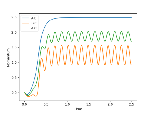
The Ising model does not take into account the energy required to change the total magnetic field generated by the lattice, so there is no activation barrier for the spin flipping process. It means that below the Curie point, where the entropic contribution is not significant, the lattice will spontaneously flip spins in order to reach the minimum energy configuration. Therefore, a spontaneous magnetization is expected. Moreover, the magnetization of the minimum energy configuration is expected, which can be 1 or -1.
 |
 |
As it can be seen in the animated plots, the energy eventually (after approx. 500 Monte Carlo steps) reaches the minimum energy (-2) and the magnetization reaches 1. However, if we look at the averages, the values will be close these values, but the random configurations generated in the beginning of the simulation slightly distort the results.
Task 9: Monte Carlo execution time
Ten time recordings were run and the result was:
t=36.259±0.392 s
Task 10: Better energy and magnetisation functions
 def energy(self):
        "Return the total energy of the current lattice configuration."
        energy = -(np.sum(np.multiply(self.lattice,np.roll(self.lattice,1,axis=0)))+np.sum(np.multiply(self.lattice,np.roll(self.lattice,1,axis=1))))
        return energy
What the new energy function does is the following:
-shifts the lattice horizontally and multiplies it by the original one
-shifts the lattice vertically and multiplies it by the original one
-adds the two resulting lattices
JC: Well noticed that you only need to use roll twice which removes double counting.
Task 11: Execution time for the new functions
Ten time recordings were run and the result was:
t=0.668±0.071 s
This improvement is incredible since the functions became roughly 50 times faster.
Task 12: Discarding some Monte Carlo cycles
After trying 8x8, 16x16, and 32x32 lattices it became apparent (as expected) that the larger the lattice the more Monte Carlo steps are needed to get the optimum configuration.
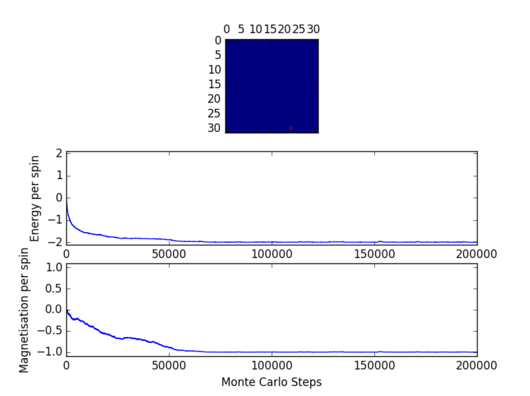 |
The above figure shows the energy and magnetization for up to 200000 Monte Carlo Steps. The optimum configuration appears to be reached after 50000-60000 steps. Therefore it would be reasonable to omit 50000 Monte Carlo steps. However, when calculations are performed for a new temperature the starting configuration will be the same as the one from the previous temperature. Therefore, if temperature steps are relatively small the two configurations will be very close, and the new configuration will be obtained after a significantly smaller number of steps. The new montecarlostep and statistics functions are presented below:
  def montecarlostep(self, T):
        # complete this function so that it performs a single Monte Carlo step
        energy0 = self.energy()
        #the following two lines will select the coordinates of the random spin for you
        random_i = np.random.choice(range(0, self.n_rows))
        random_j = np.random.choice(range(0, self.n_cols))
        #the following line will choose a random number in the rang e[0,1) for you
        self.lattice[random_i][random_j]=-self.lattice[random_i][random_j]
        energy1=self.energy()
        deltaE=energy1-energy0
        if (deltaE<=0):
            energy0=energy1
        if (deltaE>0):
            random_number = np.random.random()
            energy0=energy1
            if (random_number>np.e**(-deltaE/T)):
                self.lattice[random_i][random_j]=-self.lattice[random_i][random_j]
                energy0 = self.energy()
        magnetisation0=self.magnetisation()
        self.n_cycles+=1
        if (self.n_cycles>50000):
            self.E += energy0
            self.E2+=energy0**2
            self.M+=magnetisation0
            self.M2+=magnetisation0**2

        return [energy0,magnetisation0]

    def statistics(self):
        # complete this function so that it calculates the correct values for the averages of E, E*E (E2), M, M*M (M2), and returns them
        return [self.E/(self.n_cycles-50000),self.E2/(self.n_cycles-50000),self.M/(self.n_cycles-50000),self.M2/(self.n_cycles-50000),self.n_cycles]

'''<span style="color:red">JC: If equilibrium is reached after 50000-60000 steps, it might be better to choose to omit the maximum, 60000.  Also might be worth using a variable in the code for the number of steps to omit so that it can be easily changed if needed.</span>'''
Task 13: Adding errorbars
varM=np.array(magnetisationsq)-(np.array(magnetisations))**2
varE=np.array(energysq)-(np.array(energy))**2


enerax.errorbar(temps,np.array(energies)/spins,yerr=varE**0.5/spins)
magax.errorbar(temps,np.array(magnetisations)/spins,yerr=varM**0.5/spins)
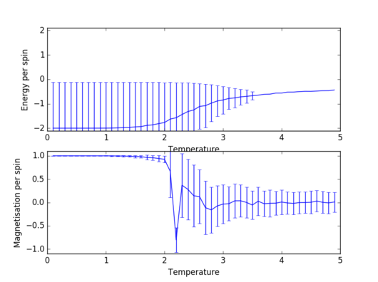
These lines were added to the ILtemperaturerange.py code in order to add the errorbars. Also, the code was set to execute 150000 Monte Carlo steps, omitting the first 50000, using a temperature step of 0.1.
 |
Task 14: Size dependence of energy and magnetisation
 |
 |
 |
 |
 |
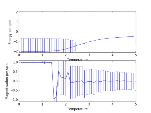
As expected, for every lattice size there are almost no fluctuations below the Curie temperature (ground state is largely favoured). As temperature gets close to the Curie point, the fluctuations become quite large, a fact indicated directly by the size of the errorbars. At a temperature higher than the Curie temperature, however, the system becomes paramagnetic2, so the number of favoured states is still significantly larger than in the case of low temperatures. However, these fluctuations are negligible for large sizes of the lattice; the 32x32 lattice already shows significantly smaller fluctuations in the paramagnetic region than an 8x8 lattice.
JC: How can you tell there are no fluctuations below the Curie temperature and why are the error bars so large for these temperatures? Why are the energy error bars at low temperature very large, but the magnetisation error bars are much smaller?
Task 15: An expression for heat capacity
The heat capacity can be calculated by expressing the expectation value of energy in terms of the energies Ei of all microstates (i=1, 2 ...).
Also, to be able to manipulate this equation we have to write the partition function explicitly. More specifically, we need to know how it depends on temperature.
Substituting this into the expression for heat capacity we get:
JC: Nice, clear derivation.
Task 16: Visualising heat capacity
The following piece of code was written in order to plot heat capacities against temperature.
import numpy as np
import matplotlib.pyplot as plt
from scipy.constants import k

temps2,energies2,energysq2,magnetisation2,magnetisationsq2=np.loadtxt("2x2.dat",unpack=True)
temps4,energies4,energysq4,magnetisation4,magnetisationsq4=np.loadtxt("4x4.dat",unpack=True)
temps8,energies8,energysq8,magnetisation8,magnetisationsq8=np.loadtxt("8x8.dat",unpack=True)
temps16,energies16,energysq16,magnetisation16,magnetisationsq16=np.loadtxt("16x16.dat",unpack=True)
temps32,energies32,energysq32,magnetisation32,magnetisationsq32=np.loadtxt("32x32.dat",unpack=True)
var2E=energysq2-energies2**2
var4E=energysq4-energies4**2
var8E=energysq8-energies8**2
var16E=energysq16-energies16**2
var32E=energysq32-energies32**2
heatcap2=var2E/(k*temps2**2)
heatcap4=var4E/(k*temps4**2)
heatcap8=var8E/(k*temps8**2)
heatcap16=var16E/(k*temps16**2)
heatcap32=var32E/(k*temps32**2)
plt.plot(temps2,heatcap2,label='2x2')
plt.plot(temps4,heatcap4,label='4x4')
plt.plot(temps8,heatcap8,label='8x8')
plt.plot(temps16,heatcap16,label='16x16')
plt.plot(temps32,heatcap32,label='32x32')
plt.legend(loc='upper right')
plt.xlabel('Temperature')
plt.ylabel('C')
plt.show()
For each of the lattice sizes the code starts by extracting the data from the files where they were saved. Then it calculates the varience using the average energy and average square energy and substitutes it into the formula derived for task 15. Finally, thecurves for 5 different lattice sizes, 2x2, 4x4, 8x8, 16x16 and 32x32, are plotted on the same graph.
 |
It is known from the work of Onsager that heat capacity at the Curie temperature diverges for infinite lattices, but an increasing peak value with lattice size is not exactly what the graph displays. This is because the number of Monte Carlo steps is not large enough to deal with the large fluctuations around the Curie point. However,, from figure 11 one can infer that for a larger lattice the curve becomes sharper around the peak, allowing for a more accurate estimate of the Curie temperature.
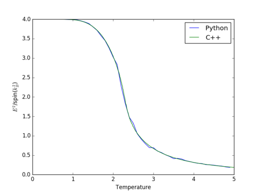
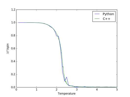
Task 17: Comparison to C++
The Python code four comparison of the four parameters is given below for a 32x32 lattice. The codes for the other lattice sizes are, of course, very similar to the one presented here:
import numpy as np
import matplotlib.pyplot as plt
from scipy.constants import k

temps32,energies32,energysq32,magnetisation32,magnetisationsq32=np.loadtxt("32x32.dat",unpack=True)
var32E=energysq32-energies32**2
heatcap32=var32E/(temps32**2)

ctemps32,cenergies32,cenergysq32,cmagnetisation32,cmagnetisationsq32,cheatcap32=np.loadtxt("bs32x32.dat",unpack=True)
plt.figure(1)
plt.plot(temps32,heatcap32/1024,label='Python')
plt.plot(ctemps32,cheatcap32,label='C++')
plt.legend('upper right')
plt.xlabel('Temperature')
plt.ylabel('C/spin(k_B)')

plt.figure(2)
plt.plot(temps32,energies32/1024,label='Python')
plt.plot(ctemps32,cenergies32,label='C++')
plt.legend('upper right')
plt.xlabel('Temperature')
plt.ylabel('E/spin(k_B)')

plt.figure(3)
plt.plot(temps32,energysq32/1024**2,label='Python')
plt.plot(ctemps32,cenergysq32,label='C++')
plt.legend('upper riught')
plt.xlabel('Temperature')
plt.ylabel('$E^2$/spin($k_B^2$)')
plt.figure(4)
plt.plot(temps32,magnetisation32/1024,label='Python')
plt.plot(ctemps32,cmagnetisation32,label='C++')
plt.legend('upper right')
plt.xlabel('Temperature')
plt.ylabel('M/spin')

plt.figure(5)
plt.plot(temps32,magnetisationsq32/1024**2,label='Python')
plt.plot(ctemps32,cmagnetisationsq32,label='C++')
plt.legend('upper right')
plt.xlabel('Temperature')
plt.ylabel('$M^2$/spin')

plt.show()
 |
 |
 |
 |
 |
The two simulations agree incredibly well in general. However,significant discrepancies between them appeat for heat capacity and magnetisation around the Curie temperature. The reason that happens is because in the vicinity of the Curie temperature there are more fluctuations and therefore, a larger number of Monte Carlo steps gives a better apprximation.
JC: Correct.
Task 18: Polynomial fitting
The following piece of code reads from the text file "bs64x64.dat" and plots both the raw data and the fitted polynomial function on the same graph.
import numpy as np
import matplotlib.pyplot as plt

T,E,E2,M,M2,C = np.loadtxt("bs64x64.dat",unpack=True)
fit = np.polyfit(T, C, 15)

T_min = np.min(T)
T_max = np.max(T)
T_range = np.linspace(T_min, T_max, 1000)
fitted_C_values = np.polyval(fit, T_range)

plt.plot(T,C,label='Raw data')
plt.plot(T_range,fitted_C_values, label='Fitted polynomial')
plt.legend(loc='upper right')
plt.show()
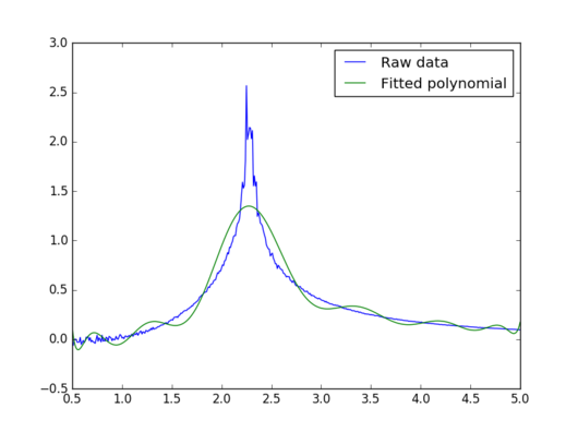 |
The polynomial fit does not appear to be good around the peak, which is the region of interest. Increasing the degree of the polynomial up to 50 does not produce a satisfactory result either. Therefore, a better way of fitting the polynomial is needed.
Task 19: Better fit
import numpy as np
import matplotlib.pyplot as plt

T,E,E2,M,M2,C = np.loadtxt("bs64x64.dat",unpack=True)

T_min = np.min(T)
T_max = np.max(T)
T_range = np.linspace(T_min, T_max, 1000)

Tminn = 2.0
Tmaxx = 3.0

selection = np.logical_and(T > Tminn, T < Tmaxx)
peak_T_values = T[selection]
peak_C_values = C[selection]

fit = np.polyfit(peak_T_values, peak_C_values, 50)
fitted_C_values = np.polyval(fit, T_range)

plt.plot(T,C,label='Raw data')
plt.plot(T_range,fitted_C_values, label='Fitted polynomial')
plt.legend(loc='upper right')
plt.ylim(0,3)
plt.show()
This modified version of the code from task 18 fits a polynomial of degree 50 this time, using temperture values between 2.0 and 3.0 and the corresponding heat capascity values.
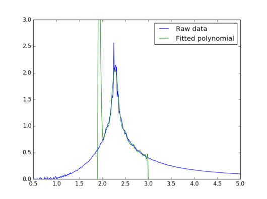 |
This new fit is very good in the peak region, so it should be very good for estimating the Curie temperature
JC: Good.
Task 20: Curie Temperature of an infinite lattice
import numpy as np
import matplotlib.pyplot as plt

files=["bs2x2.dat","bs4x4.dat","bs8x8.dat","bs16x16.dat","bs32x32.dat","bs64x64.dat"]
TC=[]
for i in files:
    T,E,E2,M,M2,C = np.loadtxt(i,unpack=True)

    T_min = np.min(T)
    T_max = np.max(T)
    T_range = np.linspace(T_min, T_max, 1000)

    Tminn = 2.0
    Tmaxx = 3.0

    selection = np.logical_and(T > Tminn, T < Tmaxx)
    peak_T_values = T[selection]
    peak_C_values = C[selection]

    fit = np.polyfit(peak_T_values, peak_C_values, 50)
    fitted_C_values = np.polyval(fit, T_range)

    Cmax = np.max(fitted_C_values)
    Tc = T_range[fitted_C_values == Cmax]
    TC+=[Tc]
length=[]
for i in range(1,7):
    length+=[2**i]
data=np.column_stack((length,TC))
np.savetxt("Curie_temps", data)

fitt = np.polyfit(np.array(length)**(-1), TC, 1)
plt.plot((np.array(length)),TC, marker='o', linestyle='')
plt.plot((np.array(length))**(-1),fitt[0]/(np.array(length))+fitt[1])
plt.show()
The code written above fits a polynomial of degree 50 to the peak region (T=2.0-3.0) of the heat capacity curves for each of the 6 lattices. Therefore, 6 fits are obtained. The maxima of these fits are taken as the Curie temperatures of the corresponding lattices. These values, together with a generated list of lattice sizes, are written to a text file called "Curie_temps.dat". These Curie temperatures are then plotted against the sizes of our lattices.
JC: How did you find the maxima of the fit?
 |
In theory the dependence of Curie temperature on lattice size is hyperbolic. Unfortunately, the points corresponding to the 4x4 and 16x16 lattices are way off. Most likely, for those simulations the large fluctuations around the Curie temperature generated an error that did not average out once the fitting was done. In any case, a fitting for these results would probably be useless. If these two points are ignored,the other for seem to follow a hyperbolic decay. Also, when the lattice size becomes very large, the decay becomes almost linear. Therefore, just by eye, one can tell that from this simulation, the Curie temperature of an infinite lattice is between 2.0 and 2.5 J/k. This is pretty close to the real value, which is 2.25 J/k. 3
JC: Plot 1/L rather than L (system size) against Curie temperature to get a straight line whose intercept gives the Curie temperature of the infinite lattice.
References
1. S. M. Bhattacharjee and A. Khare, 1995
2. P. Dobis, J. Bruestlova and M. Bartlova, 3rd Int. Symp. Eng. Educ., 2010
3. D. A. Ajadi, L. A. Sunmonu, O. A. Aremu and J. A. Oladunjoye, 2014, 9, 1336-1344
