Talk:Mod:343GLTSPRK

JC: General comments: Report is well written and the results look good. Make sure you understand the background theory behind the tasks in the experiment, especially in the analysis of the radial distribution function.

Molecular Dynamics Simulations

Introductory Theory

Velocity-Verlet Solution versus Analytical Solution for a Simple Harmonic Oscillator

The Velocity-Verlet algorithm is a numerical method of calculating the position and velocity of a particle after a specified timestep. It can be repeated over multiple timesteps to calculate how the position and velocity of any particular particle in a system evolves with time.

Figure 1. Graph of displacement vs Time, showing both the positions from the analytical solution, and from the Velocity-Verlet solution, for a timestep of 0.1 s.

Figure 2. Graph of total energy vs time, calculated from the Verlet-Velocity positions, for a timestep of 0.1 s.

Figure 3. Graph of total Error in Velocity-Verlet calculated positions (compared with analytically calculated positions) vs time, for a timestep of 0.1 s.

Figure 4. Graph of error in position maxima vs time

Velocity-Verlet Algorith

(1)${\mathbf{v}}_i(t+\frac{1}{2}\delta t)={\mathbf{v}}_i\left(t\right)+\frac{1}{2}{\mathbf{a}}_i\left(t\right)\delta t$

(2)${\mathbf{x}}_i(t+\delta t)={\mathbf{x}}_i\left(t\right)+{\mathbf{v}}_i(t+\frac{1}{2}\delta t)\delta t$

(3)${\mathbf{v}}_i(t+\delta t)={\mathbf{v}}_i(t+\frac{1}{2}\delta t)+\frac{1}{2}{\mathbf{a}}_i(t+\delta t)\delta t$

Once the initial position and velocity are specified, time is moved forward by a half step, and equation (1) is used to calculate the velocity after the half step is complete. This velocity is then used in equation (2) to calculate the new positions of the particles after the half step. The particle will be feeling new forces due to its new position, and so a new acceleration is calculated, and the full step velocity is calculated using equation (3). The process is then repeated.

The advantage of the Velocity-Verlet algorithm is that it can be used in an N-body system, which would not be possible if an analytical solution was used. This is because the velocity-Verlet algorithm uses a timestep, meaning it only has to calculate the forces on particles at instantaneous moments between specified timesteps, rather than continuously. Naturally, this leads to error, and means the algorithm can only provide and approximation of what is occurring. The smaller the the timestep however, the smaller the error, and theoretically, if the timestep were reduced to zero, the simulation would be accurate to reality. However, as timestep is decreased, calculation time is also increased. It is therefore necessary to strike a balance between how accurate the simulation needs to be, and how much calculation time one can afford. The following section displays this error-timestep dynamic.

Velocity-Verlet when applied to SHM

A simple harmonic oscillator is simply a system were the force on a particle is described by the relationship $F=-k{x}^2$, where $x$ is the position of the particle, and $k$ is a force constant. The analytical solution to the position of the particle in SHM is $x\left(t\right)=A\cos (\omega t+\varphi )$ (where $A$ is the amplitude, $\omega$ is the angular velocity, and is the phase constant. For these calculations $A=1$, $\omega =1$, and ). Now a comparison in results between using the Velocity-Verlet algorithm to calculate the values of the system versus using the analytical solution will made. It is important to realise that it is completely possible to calculate the motion of a single particle undergoing SHM analytically, but the Velocity-Verlet algorithm is being used for the sake of comparison.

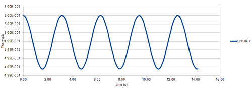
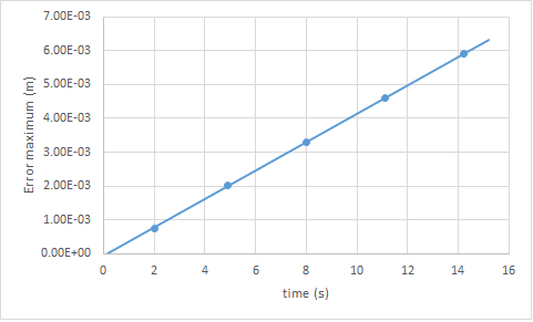
Figure 1 shows that for a timestep of 0.1 s, the error in position is in fact very small when using the Velocity-Verlet algorithm. Figure 3. shows that the error oscillates with the system, with the maximum error being when the particle is close to the origin, and the minimum being when it is at a maximum. This is of course due to the fact that error has a greater effect when smaller values are involved. It can also be seen that the error maxima increase with time. This is because the evolution of a system is dependent on its starting conditions, and as time passes, the error in the velocity-verlet solution compounds and deviates further and further from the position in the analytical solution. This can be seen in figure 4.

In figure 2. one can see that the total energy of the system (sum of PE and KE) varies with time under the velocity-verlet algorithm. This is obviously not accurate to reality, as total energy should remain constant in a closed system. This shows the disadvantages of using an approximate calculation. The error is small though, and in order to have the total energy change by 1% or less, the timestep has to be equal to 0.2 or less, which is not that small, showing that the velocity-verlet algorithm does provide a good approximation for not too much calculation time. It is important to monitor the energy of a system when modelling it in this way, because how the energy varies with the course of the simulation will provide a good idea of how accurate the simulation is.

JC: In theory the total energy should not vary over the course of the simulation (conservation of energy), so need to choose a timestep that keeps energy fluctuation down to a minimum. In the harmonic oscillator, F = kx not x^2.

Lennard-Jones Potential

LAAMPS calculates pairwise interactions between particles by modelling the force field around each particle using the Lennard-Jones potential with paramters appropriate to whatever atom is being considered. The Lennard-Jones Potential takes the following form: $\varphi \left(r\right)=4ϵ(\frac{{\sigma }^{12}}{r^{12}}-\frac{{\sigma }^6}{r^6})$ Where $\varphi \left(r\right)$ is the potential and $r$ is the separation.

Finding the separation where energy is $0$, $r_0$:

$4ϵ(\frac{{\sigma }^{12}}{r_0^{12}}-\frac{{\sigma }^6}{r_0^6})=0$

$r_0^6={\sigma }^6$

$r_0=\sigma$

Finding the force at $r_0$:

$\mathbf{F}=-\frac{\mathrm{d}U}{\mathrm{d}\mathbf{r}}$

Differentiate Lennard-Jones Potential to find force:

$\frac{\mathrm{d}\varphi \left(r\right)}{\mathrm{d}\mathbf{r}}=4ϵ(-\frac{12{\sigma }^{12}}{r^{13}}+\frac{6{\sigma }^6}{r^7})$

Substitute in $r_0=\sigma$

$F_0=\frac{-24ϵ}{\sigma }$

Finding equilibrium separation $r_{eq}$:

At equilibrium separation, potential will be at a minimum. To find the minimum, set the Lennard-Jones potential differential to 0.

$4ϵ(-\frac{12{\sigma }^{12}}{r^{13}}+\frac{6{\sigma }^6}{r^7})=0$

$r_{eq}^6=2{\sigma }^6$

$r_{eq}=1.225\sigma$

Finding Well Depth $\varphi (r_{eq})$:

Substitute $r_{eq}$ into $\varphi \left(r\right)$

$\varphi (r_{eq})=-1.9375ϵ$

Evaluating the integrals $\underset{2\sigma }{\overset{\mathrm{\infty }}{\int }}\varphi \left(r\right)\mathrm{d}r$, $\underset{2.5\sigma }{\overset{\mathrm{\infty }}{\int }}\varphi \left(r\right)\mathrm{d}r$, and $\underset{3\sigma }{\overset{\mathrm{\infty }}{\int }}\varphi \left(r\right)\mathrm{d}r$ when $\sigma =ϵ=1.0$:

Integrate $\varphi \left(r\right)$ and substitute in $\sigma =ϵ=1.0$

$\int 4ϵ(\frac{{\sigma }^{12}}{r^{12}}-\frac{{\sigma }^6}{r^6})=[-\frac{4}{11r^{11}}+\frac{4}{5r^5}]$

Apply limits of the different integrals

$\underset{2\sigma }{\overset{\mathrm{\infty }}{\int }}\varphi \left(r\right)\mathrm{d}r=-2.48\times 10^{-2}$

$\underset{2.5\sigma }{\overset{\mathrm{\infty }}{\int }}\varphi \left(r\right)\mathrm{d}r=-8.18\times 10^{-3}$

$\underset{3\sigma }{\overset{\mathrm{\infty }}{\int }}\varphi \left(r\right)\mathrm{d}r=-3.29\times 10^{-3}$

JC: The well depth should be epsilon, substitute the exact value of r_eq = 2^(1/6)*sigma into phi.

Estimating the number of water molecules in 1ml of water under standard conditions.

The molecular weight of water is 18, meaning 1 mole of water weighs 18 g. One can therefore approximate that one molecule of water weighs $\frac{18g}{N_A}$

The weight of one molecule of water is therefore approximately $2.99\times 10^{-23}g$

The density of water under standard conditions is 1 g/mL, so the number of molecules of water in 1 mL will be approximately $\frac{1g}{2.99\times 10^{-23}g}$

This gives approximately $3.34\times 10^{22}$ molecules of water in 1 mL of water.

Estimating the volume of 10000 water molecules under standard conditions:

The volume of one water molecule will be the 1 mL divided by the number of water molecules of in 1 mL of water.

$\frac{1mL}{3.34\times 10^{22}}=2.99\times 10^{-23}mL$

The volume of 1000 water molecules will be the volume of one water molecule multiplied by 1000.

$2.99\times 10^{-23}mL\times 1000=2.99\times 10^{-19}mL$

Periodic Boundary Conditions

When periodic boundary conditions are applied in a system confined to a box with dimensions 1.0 by 1.0 by 1.0, a particle crossing the edge of the box will appear on the opposite side from which it existed. Given this, consider an atom at (0.5,0.5,0.5). If this atom moves by the vector (0.7,0.6,0.2) it will, somewhat counter-intuitively, end up at the coordinates (0.2,0.1,0.7).

JC: Correct.

Reduced Units

When considering Lennard-Jones interactions, reduced units are often used as they are much more convenient than regular units. It is however important to be able to convert between them, and SI units. Given this, the conversions of the LJ cutoff, the well-depth, and the temperature, from reduced units to SI units is carried out.

$r^{*}=3.2$ $r=r^{*}\times \sigma$ $r=3.2\times 0.34nm=1.088nm$

$\frac{ϵ}{k_b}=120K$ $k_b=1.38\times 10^{-23}J{K}^{-1}$ $ϵ=120\times 1.38\times 10^{-23}=1.656\times 10^{-21}J$

$E=E^{*}\times ϵ$

$\varphi (r_{eq})=1.656\times 10^{-21}\times -1.9375=-3.2085\times 10^{-21}J=-1.9315kJmo{l}^{-1}$

$T=\frac{T^{*}ϵ}{k_b},T^{*}=1.5$

$T=1.5\times 120=180K$

JC: Correct.

Output of First Simulations

Figure 5. Graph showing how the total energy of the system varies with time for a timestep of 0.001.

Figure 6. Graph showing how the temperature of the system varies with time for a timestep of 0.001.

Figure 7. Graph showing how the pressure of the system varies with time for a timestep of 0.001

Figure 8. Graph showing how the total energy of the system varies during equilibration for simulations using different timesteps (shown in the legend).

Creating the simulation box

Starting Coordinates

When generating the starting positions of atoms for a disordered system like a liquid or gas, one needs to find a way of generating them in a disordered way. One could create a script to generate atoms at random positions, however this would pose a problem. If two atoms are randomly generated very close together, they will start with a very high potential energy, which will be converted into kinetic energy, and the temperature of the system will be higher than intended. This kind of issue would cause control of thermodynamic parameters in the simulation to be unreliable. A better way to generate starting positions is to simulate the atoms starting in their crystal lattice structure, and then allow the lattice to "melt". once the system is equilibrated, the positions of the atoms can be used to start another simulation.

JC: High repulsive forces in the initial system can cause the simulation to be unstable and to crash or require a much smaller timestep than normal.

Lattice spacing and density

In order to obtain the lattice spacing, all one needs to specify is the lattice type, and the number density.

For example if the lattice density is 0.8, and the lattice type is simple cubic. There are 0.8 lattice points per unit volume. There is one lattice point per unit cell. The volume for one lattice point will be 1.25 volume units. The lattice is simple cubic (all sides are the same length) so one must simply take the cube root of 1.25 which is 1.07722.

Another example could be a lattice density of 1.2, with a face centered cubic lattice type. The volume for one lattice point would be 5/6. An FCC lattice has 4 lattice points per unit cell. The volume for one unit cell would then be $\frac{5}{6}\times 4=\frac{10}{3}$. Once again the unit cell is cubic so all the sides are the same length, so taking the cube root of 10/3 gives a lattice spacing of 1.4938.

Creating an orthogonal box 10 x 10 x 10 unit simple cubic cells long would create a box containing 1000 unit cells. Using the create_atoms on this box will create 1000 atoms because the simple cubic lattice type only has 1 atom per unit cell. Using the same command on a 10 x 10 x 10 box of FCC unit cells would create 4000 atoms because there are 4 atoms per FCC unit cell.

JC: Correct.

Setting the Properties of the Atoms

There are three commands important in setting the properties of a type of atom.

mass 1 1.0

This simply means that the mass of atom type 1 is equal to 1.0

pair_style lj/cut 3.0

Pair-Style command tells LAMMPS how to compute the interaction between two atoms. lj/cut 3.0 means to use a Lennard-Jones potential to model the interaction, and for the potential to have a cut off radius at a distance of 3.0 from the atom.

pair_coeff * * 1.0 1.0

The pair_coeff command specifies the parameters of interactions between pairs of particles. In this case there is only one type of atom so there is only one pair, so the double * can be used. The two 1.0s specify the parameters of the Lennard-Jones (that is $ϵ$ and $\sigma$) potential for the atom pairing.

Because $x_i(0)$ and $v_i(0)$ are being specified at the start of this simulation, the Velocity-Verlet algorithm must be used.

JC: Correct.

Running the Simulation

One might pose the question, why is it important to set the timestep as a variable in the code? Why are variables used at all for that matter. The reason is that asking the code to call upon a predefined variable allows flexibility in the code e.g. if one wanted to change the timestep, all they would need to do is change the definition of the variable instead of changing many numbers separately.

JC: Good explanation.

Checking Equilibration

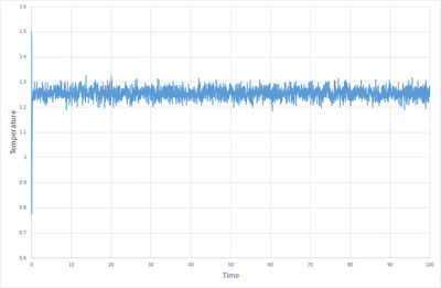
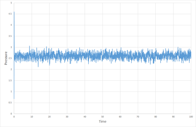
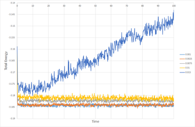
Figures 1, 2 and 3. show how the total energy, temperature and pressure vary with time from the start of the simulation when the timestep is 0.001. As can be seen, the system equilibrates in about 0.3 s. At this point one must ask the question, is a time step as small as 0.001 necessary? Figure 8 shows the total energy versus time for multiple timesteps. This shows that timesteps of 0.001 and 0.0025 give essentially the same result, and both equilibrate nicely. Timesteps of 0.0075 and 0.1 start to show discrepancies in the total energy once equilibration is complete, but they do equilibrate. When the timestep is as high as 0.015 however, the system fails to quilibrate at all, and the total energy increases with time. From this it can be deduced that a time step of 0.0025 is the maximum timestep that can be used without affecting the accuracy of the system to a great degree, and so this is the optimum timestep. Timesteps of 0.0075 and 0.01 could suffice for some purposes, but a timestep of 0.015 is not useful in any situation.

JC: Good choice of timestep.

Thermostats and Barostats

In molecular dynamics simulation, there is a target temperature

$\tau$

, and an instantaneous temperature

$T$

, which is calculated at the end of every timestep.

$T$

is rarely the same as

$\tau$

. In order to account for this, we create the velocity correction factor

$\gamma$

which we can use to change

$T$

to

$\tau$

by multiplying the velocity of every particle by this factor. This correction factor can be determined by solving the following equation for

$\gamma$

:

Figure 9. Graph showing how the density of the system varies with temperature while under constant pressure. Plots for P=2.5 and 2.7 are shown, as well as the densities calculated by the ideal gas law at these pressures.

$\frac{1}{2}\sum _i{m}_i{v}_i^2=\frac{3}{2}N{k}_{B}T$

$\frac{1}{2}\sum _i{m}_i(\gamma v_i{)}^2=\frac{3}{2}N{k}_B\tau$

$\sum _i{m}_i{v}_i^2=\frac{3N{k}_B\tau }{{\gamma }^2}$

$\frac{1}{2}\frac{3N{k}_B\tau }{{\gamma }^2}=\frac{3}{2}N{k}_{B}T$

${\gamma }^2=\frac{\tau }{T}$

$\gamma =\sqrt{\frac{\tau }{T}}$

JC: Good derivation.

Examining the Input Script

fix aves all ave/time 100 1000 100000 v_dens v_temp v_press v_dens2 v_temp2 v_press2 run 100000

The fix command simply means a command that is applied to atoms of the system. The "all" means it applies this to all atoms. ave/time has three numbers that need to be specified. The first number (100 in this case) specifies that input values to be used in calculating the average are taken from the simulation every 100 timesteps. The second number (1000) means to use 1000 input values for calculating the average, i.e. take an input value every 100 timesteps, until 1000 input values are collected, then use these to calculate the average. The final number (100000) indicates how many timesteps will pass before an average is calculated. So summing up the three numbers in this case, an input value is collected every 100 timesteps, until 1000 input values are collected, at which point the average is calculated after the passage of 100000 timesteps.

Plotting Equations of State

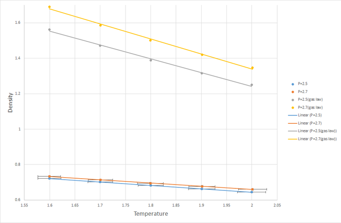
Ten simulations were carried out: 5 with a pressure of 2.5, and 5 temperatures ranging from 1.6 to 2, and another 5 with a pressure of 2.7, and 5 temperatures ranging from 1.6 to 2. The results were then used to calculate the density vs T for each of these simulations using the ideal gas law

$\frac{N}{V}=\frac{P}{kT}$

.

Figure 10. Graph of $\frac{C_V}{V}$ verus temperature at the densities 0.2 and 0.8.

As expected, the density of the systems at both pressures decrease as temperature increases, due to the volume of the simulation box expanding to accommodate the tendency for the system to increase in pressure. The density of the system fixed at P=2.7 is higher than the density of the system fixed at P=2.5. This also makes sense as a higher pressure will lead to the particles being closer together on average - leading to higher density. What is more interesting is the discrepancy in the density predicted by the ideal gas law, and the density calculated in the simulation. The ideal gas law assumes there is no interaction between particles, the atoms have essentially zero volume. Therefore at any particular pressure an ideal gas can be compressed more than the gas modeled in molecular dynamics. This explains the much higher densities for the ideal gases. It is also interesting to notes that the ideal gas curves approach the molecular dynamics curves as temperature increases. This is because ideal gases provide a more accurate approximation of real gases at higher temperatures.

JC: Why do you fit the ideal gas data to a straight line, the equation shows that density is proportional to 1/T, not T.

Calculating Heat capacities using Statistical Physics

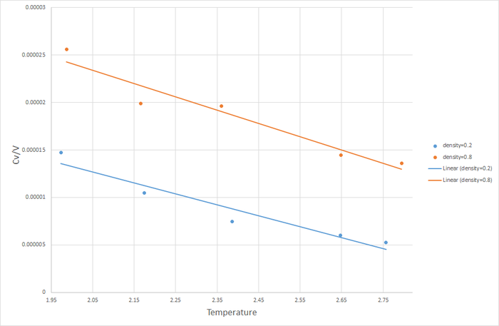
Ten simulations in density-temperature phase were carried out, at the densities 0.2 and 0.8 and the temperatures 2, 2.2, 2.4, 2.6, 2.8. This equation was used to calculate the heat capacity:$C_V=\frac{\partial E}{\partial T}=\frac{\mathrm{V}\mathrm{a}\mathrm{r}\left[E\right]}{k_B{T}^2}=N^2\frac{⟨E^2⟩-{⟨E⟩}^2}{k_B{T}^2}$

$\frac{C_V}{V}$ was then plotted as a function of temperature.

Figure 10. shows that at both densities the volumetric heat capacity decreases with temperature. This does not agree with reality, where the heat capacity of a substance increases with temperature due to more modes of excitation becoming available as temperature increases. This provides more modes for energy to be dumped into to, so less energy goes towards the translational kinetic energy of the particles, and hence the rate of temperature increase decreases. The reason for this disagreement with reality is unclear.

Figure 10. also shows that the gas at higher density has a higher volumetric heat capacity. This makes sense as there are more particles per unit volume when the density is higher, meaning there are more atoms which need to be provided kinetic energy to in order to increases the temperature, so it takes more energy to heat up the denser gas.

The input script for a gas of density 0.2 and temperature 2 is linked here Media:Nvt d=0.2,T=2

JC: Which modes of excitation are available to the simulation? There are no rotational or vibrational modes in this case. Good explanation of the trend in heat capacity with density.

Structural properties and the radial distribution function

Figure 12. Cube representing an FCC lattice. The closest three lattice points shown in the RDF are drawn in here.

figure 11. RDF functions for solid, liquid and gas.

Figure 13. The integrals of the RDFs for solid, liquid, and gas.

figure 14. Zoomed in region of solid RDF integral in region of first three lattice sites.

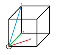
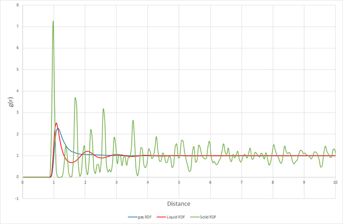
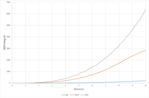
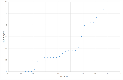
Figure 11 shows the RDF functions for a gas, a liquid, and a solid with an FCC crystal structure.

Figure 11. shows the RDFs for the simulated solid, liquid and gas. There are distinct differences in each of the RDFs. The one feature they do share in common however, is the lack of any particle density at less than approximately 1. this is because the size of the atom prevents any other atoms from approaching closer than that. Starting with the gas RDF, it shows a sudden rise in particle density at around 1, which decreases uniformly as radius increases. This uniformity of the decrease in particle density shows that the distribution of particles in a gas is random and has no structure. The liquid RDF has a peak in particle density close to the atom at about 1, then decreases before another maximum appears at approximately 2. This trend continues with the peaks getting smaller. The presence of these maxima and minima indicate that this liquid maintains some short range structure around its atoms. These could even possibly be considered "solvent shells". For the solid RDF, the structure is immediately apparent. The three peaks closest to 0 correspond to the three lattice sites shown in figure 12. Figure 13 shows the integrals of the RDFs. It can be seen that the integral for the solid increases more quickly than for the liquid, which increases more quickly than for the gas. This confirms what we already know, the solid is more dense than the liquid, which is more dense than the gas. Figure 14 shows the close up of the integration of the solid RDF in the region of the first 3 lattice sites. Using this the coordination number of each of the lattice sites can be determined. At approximately 1.1 the integration reaches 12, so the first lattice site has a coordination number of 12. After this it climbs to 18. 18-12=6, so the coordination number of the second lattice site is 6. It then climbs from 18 to 42. 42-18=24, so the coordination number of the 3rd lattice site is 24. By looking at where the integration rises sharply, it can also be determined that the lattice spacing is approximately 0.4.

JC: The third peak in the RDF is due to the atom in the centre of the face diagonally opposite the origin, not the corner atom as drawn in fig 12. Check this by calculating the number of number of nearest neighbours or the distance to this point geometrically and compare with the position of the third peak. The lattice spacing is not correct, it should be the length of the unit cell.

Dynamical properties and the diffusion coefficient

Mean Squared Displacement

The mean squared displacement of a system corresponds to the average of all the atoms in the system's displacements squared. It can be calculated using this equation:

$D=\frac{1}{6}\frac{\partial ⟨r^2\left(t\right)⟩}{\partial t}$

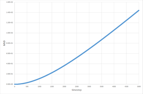
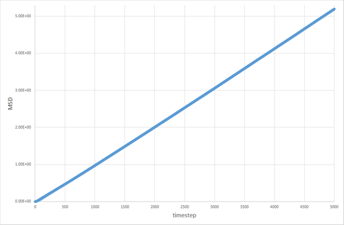
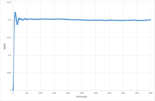
Three simulations with a timestep of 0.002 were run. A solid with density=2 and temperature=0.1, a liquid with density=0.8 and temperature=1.2, and a gas with density=0.05 and temperature=1.2 were simulated.

The table below shows the graphs of the MSD vs timestep for solid, liquid and gas simulations, run with 8000 atoms and with 1 million atoms. The diffusion coefficients associated with each graph are also shown. The graphs show that $D$ for the gases is an order of magnitude higher than for the liquids. The diffusion coefficient for solids is essentially non-existant on these time frames. This is exactly the kind of behavior one would expect. Particles in a gas have a much higher velocity than particles in a liquid, which in turn have a far higher velocity than particles in a solid, so the trend in diffusion coefficients makes sense. The value of 0 for $D$ in the solid makes sense, because in the solid the particles are locked in place in a lattice and cannot move (after equilibration has occurred) therefore their displacement would be non-existant.

The discrepancy between the 1 million and 8000 atom simulations is only truly evident in the simulation of the solid. The MSD appears to fluctuate significantly in the 8000 atom solid simulation, whereas no similar pattern is observable in the 1 million atom simulation after equilibration. This can be attributed to the random thermal vibrations in the lattice occasonally lining up to create an overall displacement. The likelihood of this occurring is higher when the number of atoms is smaller, hence why it is not seen to the same extent in the 1 million atom simulation.

	8000 atom simulation	1 million atom simulation
Gas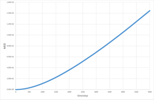
$D$	$0.006067$	$0.006033$
Liquid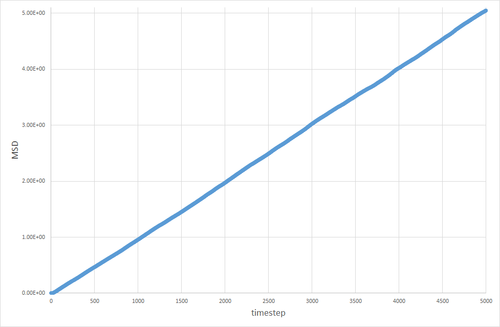
$D$	$0.000167$	$0.000167$
Solid
$D$	$0$	$0$

JC: Plot the line of best fit that you used to calculate D as well.

Deriving the normalised velocity autocorrelation function for a 1D harmonic oscillator

Figure 21. Graph showing VACFs against timestep for the simulated liquid, solid and a simple harmonic system.

Autocorrelation function: $C\left(\tau \right)=\frac{\underset{-\mathrm{\infty }}{\overset{\mathrm{\infty }}{\int }}v\left(t\right)v(t+\tau )\mathrm{d}t}{\underset{-\mathrm{\infty }}{\overset{\mathrm{\infty }}{\int }}{v}^2\left(t\right)\mathrm{d}t}$

simple harmonic oscillator: $x\left(t\right)=A\cos (\omega t+\varphi )$

$\frac{\mathrm{d}x(t)}{\mathrm{d}t}=v(t)$

differentitate harmonic oscillator equation

$v(t)=-A\omega \sin (\omega t+\varphi )$

$v(t+\tau )=-A\omega \sin (\omega (t+\tau )+\varphi )$

Substitute these into the Autocorrelation function

$C\left(\tau \right)=\frac{\underset{-\mathrm{\infty }}{\overset{\mathrm{\infty }}{\int }}(-A\omega \sin (\omega t+\varphi ))(-A\omega \sin (\omega (t+\tau )+\varphi ))\mathrm{d}t}{\underset{-\mathrm{\infty }}{\overset{\mathrm{\infty }}{\int }}{A}^2{\omega }^{2}si{n}^2(\omega t+\varphi )\mathrm{d}t}$

$A$s and $\omega$s cancel

$C\left(\tau \right)=\frac{\underset{-\mathrm{\infty }}{\overset{\mathrm{\infty }}{\int }}(\sin (\omega t+\varphi ))(\sin (\omega (t+\tau )+\varphi ))\mathrm{d}t}{\underset{-\mathrm{\infty }}{\overset{\mathrm{\infty }}{\int }}si{n}^2(\omega t+\varphi )\mathrm{d}t}$

Use trigonometric identity $\sin (A+B)=\sin (A)\cos (B)+\cos (A)\sin (B)$

$C\left(\tau \right)=\frac{\underset{-\mathrm{\infty }}{\overset{\mathrm{\infty }}{\int }}(\sin (\omega t+\varphi ))(\sin (\omega +\varphi )\cos (\omega t)+\cos (\omega t+\varphi )\sin (\omega \tau ))\mathrm{d}t}{\underset{-\mathrm{\infty }}{\overset{\mathrm{\infty }}{\int }}si{n}^2(\omega t+\varphi )\mathrm{d}t}$

Take constants out of integration

$C\left(\tau \right)=\frac{\cos (\omega t)\underset{-\mathrm{\infty }}{\overset{\mathrm{\infty }}{\int }}{\sin }^{}(\omega t+\varphi )+\sin (\omega \tau )\underset{-\mathrm{\infty }}{\overset{\mathrm{\infty }}{\int }}\sin (\omega t+\varphi )\cos (\omega t+\varphi )\mathrm{d}t}{\underset{-\mathrm{\infty }}{\overset{\mathrm{\infty }}{\int }}si{n}^2(\omega t+\varphi )\mathrm{d}t}$

$C\left(\tau \right)=\cos (\omega \tau )+\frac{\sin (\omega \tau )\underset{-\mathrm{\infty }}{\overset{\mathrm{\infty }}{\int }}\sin (\omega t+\varphi )\cos (\omega t+\varphi )\mathrm{d}t}{\underset{-\mathrm{\infty }}{\overset{\mathrm{\infty }}{\int }}si{n}^2(\omega t+\varphi )\mathrm{d}t}$

The function $\sin (\omega t+\varphi )\cos (\omega t+\varphi )$ is odd (odd multiplied by even is odd), and so when integrated between $-\mathrm{\infty }$ and $\mathrm{\infty }$ it becomes 0 leaving only one term:

$C\left(\tau \right)=\cos (\omega \tau )$

JC: Good, clear derivation.

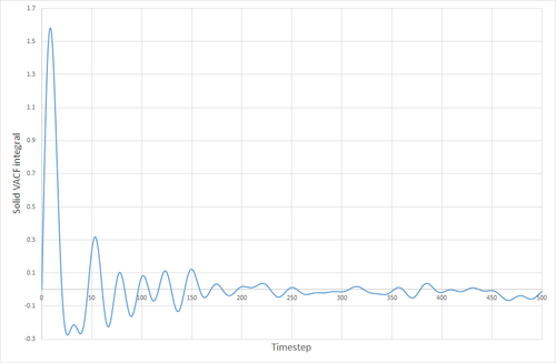
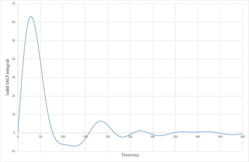
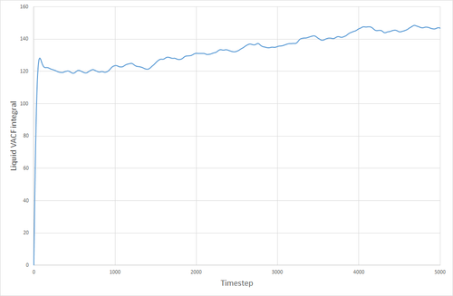
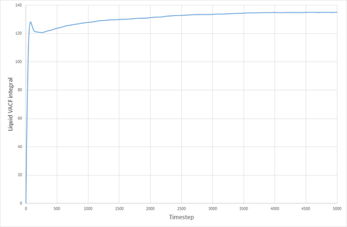
The VACF curves for the solid and the liquid simulations show different features. The solid curve starts with a small positive value, indicating that the velocities of the particles in the solid correlate well with the initial velocity that was specified for the particles. This dips below zero meaning that the particles now collectively have a velocity that is in the opposite direction to their original velocity. The particles' velocity oscillates back and forth like this, until the concerted velocity of the particles is lost, and their velocities begin to take on a more random appearance. This corresponds to the size of the maxima ad minima decreasing with time. The liquid VACF starts at a higher value, indicating the higher velocity of the particles in the liquid. The correlation between the particles' velocities and their initial velocities quickly is destroyed because of the less constrained and more random nature of the movement of particles in a liquid, as opposed to a solid where the particles are much more fixed, and the correlation can still be seen after a long time has passed. THE VACF of the SHM particle is very unlike those for a solid or liquid. It oscillates uniformly and in a highly predictable manner that will always correlate with its initial conditions. There is nothing in its environment that will cause the SHM to start oscillating differently either.

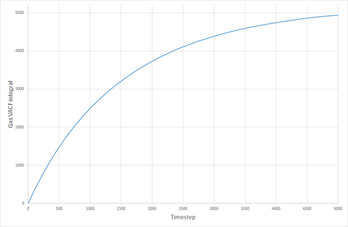
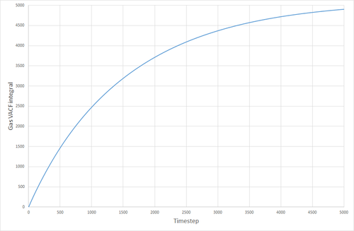
The VACF curves were integrated (see following figures) and the diffusion coefficient was calculated from their integrals. Solid, 8000 atoms: Integral=-0.00972, $D$=-0.00324 (essentially zero) Liquid, 8000 atoms: Integral=146.82, $D$=48.94 Gas, 8000 atoms: Integral=4941.95, $D$=1647 Solid, 1000000 atoms: Integral=-0.41627, $D$=-0.1388 (essentially zero) Liquid, 1000000 atoms: Integral=135.3386 $D$=45.113 Gas, 1000000 atoms: Integral=4902.765, $D$=1634.255

The values of $D$ given here are much higher than they were when derived from the MSD. The reason for this is not clear. The biggest source of error for this method of calculating the diffusion coefficient was probably the trapezium rule, although it is also possible that the model being used was not good enough, or the simulation size was too small.

Figure 15. Graph showing the running integral of the VCAF for a solid simulated with 8000 atoms.

Figure 16. Graph showing the running integral of the VCAF for a Solid simulated with 1000000 atoms.

Figure 17. Graph showing the running integral of the VCAF for a liquid simulated with 8000 atoms.

Figure 18. Graph showing the running integral of the VCAF for a liquid simulated with 1000000 atoms.

Figure 19. Graph showing the running integral of the VCAF for a gas simulated with 8000 atoms.

Figure 20. Graph showing the running integral of the VCAF for a gas simulated with 1000000 atoms.

JC: Good explanation of the VACF. The decorrelation in the VACF is due to collisions with with other particles and this is why there is no decay in the harmonic oscillator.