Talk:MOD:ZYH1018

JC: General commentsː All tasks answered and plots look good. Some of your written explanations are quite unclear though, try to make your writing more focused and concise.

Running your first simulation

This part introduces us the procedures to run simulations with a software package called LAMMPS on the High Performance Computing (HPC) systems and five example simulations with different timesteps were performed for following sections.

Introduction to molecular dynamics simulation

Numerical Integration

The Classical Particle Approximation states that in a collection of $N$ atoms, each one of them behaves as aclassical particle and will interact with others and experience a force which causes accelaration according to Newton's second law. Thus,the atomic positions and velocities at any time can be determined if the force,$F_i$ is calculated as a fuction of time $t$. By applying those theories as well as Taylor expension to "classical Verlet Algorithm", if we denote the position of an atom,$i$, at time $t$ by ${\mathbf{x}}_i\left(t\right)$, the positions of the atoms at next time step, $t+\delta t$ can be calculated by:

$$\begin{gathered} {\mathbf{x}}_i(t+\delta t)\approx 2{\mathbf{x}}_i\left(t\right)-{\mathbf{x}}_i(t-\delta t)+\frac{{\mathbf{F}}_i\left(t\right)}{m_i}\delta t^2 \\ (1) \end{gathered}$$

However, we cannot acquire any information about the velocities which is needed for calculating the kinetic energy by classical Verlet Algorithm. Therefore, a modified one called "velocity-Verlet Algorithm" is used instead and expressed as:

$$\begin{gathered} {\mathbf{x}}_i(t+\delta t)={\mathbf{x}}_i\left(t\right)+{\mathbf{v}}_i(t+\frac{1}{2}\delta t)\delta t \\ (2) \end{gathered}$$ $$\begin{gathered} {\mathbf{v}}_i(t+\delta t)={\mathbf{v}}_i(t+\frac{1}{2}\delta t)+\frac{1}{2}{\mathbf{a}}_i(t+\delta t)\delta t \\ (3) \end{gathered}$$

For the default time step 0.1

Figure 1:　"ANALYTICAL" and the velocity-Verlet functions of the position x versus time t.

Figure 2: Functions of error between "ANALYTICAL" and the velocity-Verlet solutions and the maxima in error versus time.

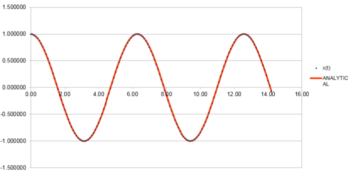
From figure 1 and figure 2 we can find that the error between "ANALYTICAL" and the velocity-Verlet solutions is quite small and the function of the error versus time is kind of "periodic" with increasing amplitudes and a half period compared to that of the position $x(t)$ of a classical harmonic oscillator, which is given by $x\left(t\right)=cos\left(t\right)$, as the error comes to zero when the $x(t)$ reaches a minimum or maximum. And the maximum value of error in each period increases linearly with time as a function of $y=0.0004x-8\times 10^{-5}$.

JC: Why does the error fluctuate?

Figure 3: Energy versus times at 0.01 timestep.

Figure 4: Energy versus times at 0.02 timestep.

Figure 5: Energy versus times at 0.024 timestep.

Figure 6: Maximum percentage change in energy versus timestep.

The energy contains the total energy of the oscillator for the velocity-Verlet solution, which is composed of kinetic energy and potential energy. Therefore,

$E_{total}=E_K+E_P=\frac{1}{2}m{v}^2+\frac{1}{2}k{x}^2$

$k=m=1$ in this case, so:

$E_{total}=\frac{{x_{(t)}}^2+{v_{(t)}}^2}{2}$

From figure 3 to figure 6 above, it can be seen that the maximum percentage change in total energy (fluctuation) increases as timestep increases. When timestep is around 0.20, the maximum change in energy is 1%. Thus, the timestep should be no more than 0.20 to ensure that the total energy does not change by more than 1%. Besides, it is important to monitor the total energy of a physical system that does not change or fluctuate too much so that the total of potential and kinetic energy is always conserved if there is no extra force applied on the system.

JC: Good, thorough analysis..

Atomic Forces

For a single Lennard-Jones interaction, the potential energy is zero when:

$\varphi \left(r_0\right)=4ϵ(\frac{{\sigma }^{12}}{r_0^{12}}-\frac{{\sigma }^6}{r_0^6})=0$

Rearrange to get:

$r_0=\sigma$

The force acting on the atom is determined by the potential it expierences:

$\mathbf{F}=-\frac{\mathrm{d}\varphi \left(\mathbf{r}\right)}{\mathrm{d}\mathbf{r}}=4ϵ(12(\frac{{\sigma }^{12}}{r^{13}})-6(\frac{{\sigma }^6}{r^7}))=24ϵ(2(\frac{{\sigma }^{12}}{r^{13}})-\frac{{\sigma }^6}{r^7})$

When $r=r_0=\sigma$:

${\mathbf{F}}_{\mathbf{(}{\mathbf{r}}_{\mathbf{0}}\mathbf{)}}=24ϵ(\frac{2}{\sigma }-\frac{1}{\sigma })=\frac{24ϵ}{\sigma }$

The equilibrium will be reached when the resultant force $F$ equals zero (the potential energy $\varphi (r)$ reaches a minimum):

${\mathbf{F}}_{\mathbf{(}}{\mathbf{r}}_{\mathbf{e}\mathbf{q}\mathbf{)}}=24ϵ(2(\frac{{\sigma }^{12}}{{r_{eq}}^{13}})-\frac{{\sigma }^6}{{r_{eq}}^7})=0$

Rearrange to get:

$\frac{{\sigma }^6}{{r_{eq}}^6}=\frac{1}{2}$

Therefore,

$r_{eq}=\sqrt[6]{2}\sigma$

And the well depth is:

$\varphi \left(r_{eq}\right)=4ϵ(\frac{{\sigma }^{12}}{{r_{eq}}^{12}}-\frac{{\sigma }^6}{{r_{eq}}^6})=4ϵ(\frac{{\sigma }^{12}}{4{\sigma }^{12}}-\frac{{\sigma }^6}{2{\sigma }^6})=-ϵ$

when $\sigma =ϵ=1.0$,

$\int \varphi \left(r\right)\mathrm{d}r=\int (\frac{4}{r^{12}}-\frac{4}{r^6})\mathrm{d}r=-\frac{4}{11r^{11}}+\frac{4}{5r^5}$

Therefore,

$\underset{2\sigma }{\overset{\mathrm{\infty }}{\int }}\varphi \left(r\right)\mathrm{d}r=0+\frac{4}{11}\times 2^{-11}-\frac{4}{5}\times 2^{-5}\approx -2.48\times 10^{-2}$

$\underset{2.5\sigma }{\overset{\mathrm{\infty }}{\int }}\varphi \left(r\right)\mathrm{d}r=0+\frac{4}{11}\times 2.5^{-11}-\frac{4}{5}\times 2.5^{-5}\approx -8.18\times 10^{-3}$

$\underset{3\sigma }{\overset{\mathrm{\infty }}{\int }}\varphi \left(r\right)\mathrm{d}r=0+\frac{4}{11}\times 3^{-11}-\frac{4}{5}\times 3^{-5}\approx -3.29\times 10^{-3}$

JC: All maths correct and well laid out.

Periodic Boundary Conditions

Under standard conditons, the density of water $\rho =1.0gm{L}^{-1}$, and the total mass of water molecules in $1mL$ of water $m=1.0g$. Therefore, the number of moles of water molecules is $n_{H_{2}O}=\frac{m_{H_{2}O}}{M_{H_{2}O}}=\frac{1.0g}{18gmo{l}^{-1}}\approx 0.056mol$.

The number of water molecules in $1mL$ of water is $N_{H_{2}O}=n_{H_{2}O}\times N_A=0.056mol\times 6.023\times 10^{23}mo{l}^{-1}\approx 3.35\times 10^{22}$.

The volume of $10000$ water molecules is $V=\frac{10000}{3.35\times 10^{22}m{L}^{-1}}\approx 3.0\times 10^{-19}mL$.

The atom at initial position $(0.5,0.5,0.5)$ moves along the vector $(0.7,0.6,0.2)$ and will reach at the final position $(0.5+0.7,0.5+0.6,0.5+0.2)$ = $1.2,1.1,0.7$ under classical conditions. But by applying the periodic boundary conditions, the atom moves in a cubic simulation box which runs from $(0,0,0)$ to $(1,1,1)$, and when it crosses the boundary of the box,one of its replicas enters the box through the opposite site. Therefore, the final position that the atom ends up should be $(1.2-1,1.1-1,0.7)=(0.2,0.1,0.7)$.

Reduced Units

When the LJ cutoff is $r^{*}=3.2$, The distance in real units should be:

$r=\sigma r^{*}=0.34nm\times 3.2=1.088nm\approx 1.1nm$

The well depth is:

$\varphi \left(r\right)=4ϵ(\frac{{\sigma }^{12}}{r^{12}}-\frac{{\sigma }^6}{r^6})N_A=4ϵ(\frac{{\sigma }^{12}}{(\sigma {r^{*})}^{12}}-\frac{{\sigma }^6}{{(\sigma r^{*})}^6})N_A=4ϵ(\frac{1}{{r^{*}}^{12}}-\frac{1}{{r^{*}}^6})N_A=4\times 120K\times K_B(\frac{1}{{r^{*}}^{12}}-\frac{1}{{r^{*}}^6})N_A$

= $4\times 120K\times 1.381\times 10^{-23}J{K}^{-1}\times (\frac{1}{{3.2}^{12}}-\frac{1}{{3.2}^6})\times 6.02\times 10^{23}mo{l}^{-1}\approx -3.71Jmo{l}^{-1}=-3.71\times 10^{-3}kJmo{l}^{-1}$

The reduced teperature $T^{*}=1.5$ in real units is :

$T=\frac{ϵ}{K_B}{T}^{*}=120K\times 1.5=180K$

JC: All calculations correct, except for the well depth. You have already shown that the well depth is just epsilon, so you just need to convert the value of epsilon given into kJmol-1.

Equilibration

Creating the simulation box

As it mentioned before, we need to specify the starting position of each atom before staring a simulation. However, it is quite hard to determine a point of reference for atoms in a liquid because there is no ordered crystal structures or unit cells. We could generate a random starting position for each atom, but this would probably cause a situation that two atoms are too close or overlapped together. And according to the Lennard-Jones potential relationship:

$\varphi \left(r\right)=4ϵ(\frac{{\sigma }^{12}}{r^{12}}-\frac{{\sigma }^6}{r^6})=0$

When the distance between two atoms are small, the potential energy will be infinitely large, which could cause a large error in simulation.

Consider a simple cubic lattice which consists of one lattice point on each corner of the cube, each atom at a lattice point is shared equally between eight adjacent cubes. So there is totally $\frac{1}{8}\times 8=1$ atom in each unit cell. When the number density is $0.8$,

number density$n=\frac{\frac{1}{8}\times 8}{1.07722^3}\approx 0.8$

,

Consider a face-centered cube which consists of one lattice point on each corner and face of the cube, each atom on the face is shared equally between rwo adjacent cubes. It gives totally $\frac{1}{8}\times 8+\frac{1}{2}\times 6=4$ atoms in each unit cell. If the number density is 1.2,

$1.2=\frac{4}{r^3}$

,

$r=\sqrt[3]{\frac{4}{1.2}}\approx 1.4938$

For the face-centered cubic lattice, each unit cell contains 4 lattice points or atoms as calculated before. Therefore, in a box that contains $1000$ unit cells of this lattice, there are $4\times 1000=4000$ atoms in total.

JC: Correct.

Setting the properties of the atoms

mass 1 1.0

this defines the mass of the single atom of type 1 is 1.0

pair_style lj/cut 3.0

The lj/cut styles computes the standard 12/6 Lennard-Jones potential, given by:

$E=4ϵ[(\frac{\sigma }{r}{)}^{12}-(\frac{\sigma }{r}{)}^6],r<r_c$

$R_c$ is the cuttoff, it equals to 3.0 in this case, which means the LJ interaction over separating distance 3.0 is negligible.

pair_coeff * * 1.0 1.0

It specifies the pairwise force field coefficients for one or more pairs of atom types, $ϵ=\sigma =1$ in this case. An asterisk means all types of atoms from 1 to N, and then the two asterisks indicate that the coefficients apply to LJ potential between any two atoms.

If initial conditions with $x_i(0)$ and $v_i(0)$ are specified, then we will apply velocity-Verlet Algorithm to run the simulation.

JC: Correct, why is a cutoff used for the potential?

Running the simulation

### SPECIFY TIMESTEP ###
variable timestep equal 0.001
variable n_steps equal floor(100/${timestep})
variable n_steps equal floor(100/0.001)
timestep ${timestep}
timestep 0.001

### RUN SIMULATION ###
run ${n_steps}
run 100000

Here we define a variable called "timestep" and thus we can just type ${timestep} in the following parts instead of the exact number. The advantage of this is that when we need to change the timestep, we only need to change the timestep number in the second line and the ${timestep} in the following parts will be changed automatically. However, if we just write:

timestep 0.001
run 100000

Once we need to change timestep, we need to change every timestep in the whole text manually.

JC: Correct.

Checking equilibration

Figure 7: Total energy versus time at a timestep 0.001

Figure 8: Temperature versus time at a timestep 0.001

Figure 9:Pressure versus time at a timestep 0.001

From figure 7 to figure 9 above, it can be seen that the energy, temperature and pressure reaches constant with small fluctuations after a short time, which indicates that the simulation reaches equilibrium. The fluctuations(error) in energy is the smallest compared to those in temperature and pressure. From the thermodynamic data of the simulation, it takes about 0.22 and 0.18 to reach the equilibrium for temperature and pressure respectively. And it takes around 0.28 for energy to reach the equilibrium just after the equilibrium of temperature and pressure.

Figure 10: Energy versus time for five different timesteps

From figure 10 we can notice that the simulations of energy at timesteps at 0.001 and 0.0025 after the equilibrium is reached are almost overlapped, and the simulations of energy at 0.0075 and 0.01 reaches equilibrium as well but with relatively higher energies compared to those at timesteps 0.001 and 0.0025, which cause larger errors or fluctuations.Therefore, the largest timestep that gives acceptable results is 0.0025. The one with the largest timestep 0.015 is a particularly bad choice because the energy increases as time increases with relative large fluctuation(error) and never reaches equilibrium. Therefore, the total energy will not be conserved.

JC: Good choice of timestep, the average total energy should not depend on the timestep.

Running simulations under specific conditions

Temperature and Pressure Control

Ten npt input files with different combinations of five tempreatures(1.6, 1.8, 2.0, 2.5, 3.0) and two pressures(2.6, 2.7) in reduced units are modified to run simulations on the HPC portal.

Thermostats and Barostats

In the system with $N$ atoms, each with three degrees of freedom, according to the equipartition theorem, we can obtained that:

$E_K=\frac{3}{2}N{k}_{B}T$ $\frac{1}{2}\sum _i{m}_i{v}_i^2=\frac{3}{2}N{k}_{B}T(4)$

After each velocity is multiplied by a constant factor $\gamma$, the temperature $T$ is corrected to $\mathfrak{𝔗}$, so:

$\frac{1}{2}\sum _i{m}_i(v_i\gamma {)}^2=\frac{{\gamma }^2}{2}\sum _i{m}_i{v}_i^2=\frac{3}{2}N{k}_B\mathfrak{𝔗}(5)$

Divide $(5)$ by $(4)$:

$\frac{\frac{{\gamma }^2}{2}\sum _i{m}_i{v}_i^2}{\frac{1}{2}\sum _i{m}_i{v}_i^2}=\frac{\frac{3}{2}N{k}_B\mathfrak{𝔗}}{\frac{3}{2}N{k}_{B}T}$

${\gamma }^2=\frac{\mathfrak{𝔗}}{T}$

Therefore,

$\gamma =\sqrt{\frac{\mathfrak{𝔗}}{T}}$

JC: Correct.

Examining the Input Script

The number "100" corresponds to $N_{every}$, which means using input values every 100 timesteps. The number "1000" corresponds to $N_{repeat}$, which means number of times to use input values for calculating averages. And the number "100000" corresponds to $N_{freq}$, which means calculating averages every this timestep. The $N_{every}$, $N_{repeat}$ and $N_{freq}$ arguments specify on what timesteps the input values will be used in order to contribute to the average. The final averaged quantities are generated on timesteps that are a multiple of $N_{freq}$. The average is over $N_{repeat}$ quantities, computed in the preceding portion of the simulation every $N_{every}$ timesteps. Therefore, in this case values on timesteps $100$, $200$, $300$, $400$, ..., $100000$ will be used to compute the final average on timestep $100000$, which means every $100$ timesteps, values of the temperature, etc., be sampled for the average. And totally $\frac{100000}{100}=1000$ measurements(the same as $N_{repeat}$) will contribute to the average. Because we need to run the simulation until reaching the final timestep $100000$, if we assume the timestep is $0.0025$, and then the total time we need to simulate is $100000\times 0.0025=250$.

JC: Good.

Plotting the Equations of State

Figure 11:Density versus temperature at pressure 2.6

Figure 12: Density versus temperature at pressure 2.6

According to the ideal gas law and reduced units conversion:

$PV=N{K}_{B}T$

$P=P^{*}\frac{ϵ}{{\sigma }^3}$

$T=T^{*}\frac{ϵ}{K_B}$

The density in reduced units can be obtained by:

${\rho }^{*}=\frac{N}{V^{*}}={\sigma }^3\frac{N}{V}={\sigma }^3\frac{P}{K_{B}T}={\sigma }^3\frac{\frac{ϵ}{{\sigma }^3}{P}^{*}}{K_B\frac{ϵ}{K_B}{T}^{*}}=\frac{P^{*}}{T^{*}}$

We use this derivation of the density in reduced units to plot graphs of density versus temperature. And it is shown from figure 11 and 12 that the simulated densities in both cases are lower that calculated by ideal gas law. This is because the ideal gas law assumes that there is no interactions between particles. But in this simulation case, there are LJ interactions between atoms, which means there could be a repulsion between atoms that repel them further apart. And the density is the number of atoms per unit volume, therefore, the simulation density is always lower than the ideal density because of the longer distances between atoms due to LJ interactions(repulsion). And as temperature increases, the density decreases. This is because the volume of the system will increase as temperature increases when pressure is constant according to the ideal gas law. Therefore, the density decreases with temperature as the total number of atoms remains the same but the volume increases.

Figure 13:Discrepancy versus temperature at pressure 2.6 and 2.7

As shown in figure 13, the density at pressure 2.7 is always higher than the density at pressure 2.6, we can consider at a given temperature and number of atoms, when pressure increases, volume will decrease according to ideal gas law, which indicates that atoms pretend to be closer and suffer greater repulsion forces due to LJ interaction, thus it will deviate more from the ideal one. Besides, the trend of the discrepancy decreases as temperature increases, this is because as temperature increases, volume increases as well if the pressure and number of atoms are constant. Therefore, atoms becomes further apart from each other and affected less from the LJ interaction, and the increased volume caused by it is less and less significant compared to the total volume, which increases as temperature increases.

JCː Explanations are correct, but a bit unclear, try to make them more concise. Joining the ideal gas data points with straight lines is misleading because the ideal gas law does not follow these lines in between data points.

Calculating heat capacities using statistical physics

below is the input script with $\rho =0.2$ and $T=2.0$ to run the simulation for heat capacity $C_V$ under $NVT$ conditions:

variable density equal 0.2

### DEFINE SIMULATION BOX GEOMETRY ###
lattice sc ${density}
region box block 0 15 0 15 0 15
create_box 1 box
create_atoms 1 box

### DEFINE PHYSICAL PROPERTIES OF ATOMS ###
mass 1 1.0
pair_style lj/cut/opt 3.0
pair_coeff 1 1 1.0 1.0
neighbor 2.0 bin

### SPECIFY THE REQUIRED THERMODYNAMIC STATE ###
variable T equal 2.0
variable timestep equal 0.0025

### ASSIGN ATOMIC VELOCITIES ###
velocity all create ${T} 12345 dist gaussian rot yes mom yes

### SPECIFY ENSEMBLE ###
timestep ${timestep}
fix nve all nve

### THERMODYNAMIC OUTPUT CONTROL ###
thermo_style custom time etotal temp press
thermo 10

### RECORD TRAJECTORY ###
dump traj all custom 1000 output-1 id x y z

### SPECIFY TIMESTEP ###

### RUN SIMULATION TO MELT CRYSTAL ###
run 10000
unfix nve
reset_timestep 0

### BRING SYSTEM TO REQUIRED STATE ###
variable tdamp equal ${timestep}*100
fix nvt all nvt temp ${T} ${T} ${tdamp} 
run 10000
reset_timestep 0

### MEASURE SYSTEM STATE ###
thermo_style custom step etotal temp vol atoms density
variable dens equal density
variable temp equal temp
variable temp2 equal temp*temp
variable volume equal vol
variable N2 equal atoms*atoms
variable E equal etotal
variable E2 equal etotal*etotal
fix aves all ave/time 100 1000 100000 v_dens v_temp2 v_E v_E2 v_N2 v_temp
unfix nvt
fix nve all nve
run 100000

variable avetemp equal f_aves[6]
variable heatcapacity equal ${N2}*(f_aves[4]-f_aves[3]*f_aves[3])/f_aves[2]
variable CperV equal ${heatcapacity}/${volume}

print "Averages"
print "--------"
print "heatcapacity: ${heatcapacity}"
print "heatcapacity/volume: ${CperV}"
print "Temperature: ${avetemp}"

The heat capacity can be calculated by the equation:

$C_V=\frac{\partial E}{\partial T}=\frac{\mathrm{V}\mathrm{a}\mathrm{r}\left[E\right]}{k_B{T}^2}=N^2\frac{⟨E^2⟩-{⟨E⟩}^2}{k_B{T}^2}(6)$

In this case, the volume is constant under $NVT$ conditions, and we will be in density-temperature $({\rho }^{*},T^{*})$ phase space, rather than pressure-temperature $(P^{*},T^{*})$phase space. Therefore, density $\rho$ is defined as a variable rather than pressure $P$.

Figure 14:Heat capacity per volume versus temperature at two densities 0.2 and 0.8 respectively

It can be seen that the heat capacity per volume decreases as temperature increases for both densities, which is consistent with the equation $(6)$. This is because as temperature increases, more atoms absorbs enough energy to reach the excited states or higher energy levels in a constant volume, which means fewer atoms on the ground state can absorb extra energy from outside. Therefore, fewer energy can be taken by the atoms in the system with constant volume and the heat capacity per volume decreases as well as temperature increases. Besides, the heat capacity per volume at density 0.8 is always higher than that at density 0.2. According to the equation: ${\rho }^{*}=\frac{P^{*}}{T^{*}}$, the pressure will be greater for a larger density if the temperature is constant. And the larger pressure and density means that atoms are closer and larger amount of atoms in a constant volume. Therefore, we can choose a constant temperature at x-axis in figure 14 and find its corresponding y values of heat capacity per volume at both densities, the one with a higher density 0.8 has a larger value because there are more atoms per unit volume that can absorb energy and be excited to higher levels, which leads to a higher heat capacity. And according to the equation $(6)$, the variance in energy $E$ increases as density increases, so the heat capacity increases.

JC: Correct explanation of the trend in heat capacity with density, the trend with temperature is harder to explain and would need more analysis beyond the scope of this experiment.

Structural properties and the radial distribution function

Figure 15: RDF g(r) versus distance r for solid, liquid and vapour phases

Phase	Density (reduced unit)	Temperature (reduced unit)	Characters and differences in RDF
Vapour	0.05	2.2	There is only one peak in RDF, which means atoms in vapour state are disordered and moving randomly. So there is no extra peaks which shows long or short rang order.
Liquid	0.8	1.2	There are three main peaks with decreasing amplitudes, and the decay rate is faster compared with that of solid. This is because the atoms in liquid phase has a short range order and has a higher degree of freedom, which means the velocity or VACF is influenced more by the distance $r$.
Solid	1.2	0.5	In solid states, atoms are highly ordered and packed closely due to the large density, and this leads to relatively high values of RDF. There are many peaks with shorter widths and decreasing amplitudes, and the decay rate is slower than that of liquid state. This is because the atoms in solid state only vibrate and have lowest degree of freedom. Therefore, the RDF is affected the least by the increasing distance. And the first three peaks correspond to short range order, the following small peaks correspond to long range order. The widths between the peaks is corresponding to the distances between atoms in the first coordination shell, second coordination shell and etc.

JC: Good, but what do you mean by "...the velocity or VACF is influenced more by the distance r."?

The graph of integral of $G(r)$ in the solid state versus distance is shown as below:

Figure 16: integral of RDF g(r) versus distance r for solid phase

And according to the FCC structure:

The first peak corresponds to the 12 atoms (colored in blue orange and green) located at the center of the $12$ faces of unit cells, which adjacent to the central reference atom(red one). The second peak corresponds to $18-12=6$ atoms (pink), which are secondly nearest to the central reference atom and located at the corners that are the most close to the reference atom. The third peak corresponds to $42-18=24$ atoms, which are located at the rest of all grey points at the center of each face of unit cell. Because these points are closer to the reference atom than those at the corner. And the lattice spacing is just the same as the distance between any one of pink atoms and the central red atom according to the FCC lattice above, therefore, the lattice spacing is equal to the distance of the second peak which $1.625$ as shown in the figure 16.

JC: Good diagram to show which atoms are responsible for the first 3 peaks. Could you have calculated the lattice parameter from the first and third peaks as well and then averaged it, how does it compare to the lattice parameter of the initial structure of your simulation?

Dynamical properties and the diffusion coefficient

Mean Squared Displacement

From simulations of my relatively small system, we can get the relationships between MSD and timestep for different phases:

Figure 17:Total MSD versus time for vapour phase

Figure 18: Total MSD versus time for liquid phase

Figure 19: Total MSD versus time for solid phase |

Acoording to the equation :

$D=\frac{1}{6}\frac{\partial ⟨r^2\left(t\right)⟩}{\partial t}$

Diffusion coefficient $D$ can be calculated if the gradient (first derivative) of the line part in each diagram of MSD versus timestep is known, as the linear relationship needs a little time to be established. And the gradient can be calculated by any two points on the linear part.Therefore:

In vapour phase, $D=\frac{1}{6}\times \frac{252-102}{9.752-5.196}\approx 5.49$

In liquid phase, $D=\frac{1}{6}\times \frac{4.76-1.21}{4702-1243}\approx 0.086$

In solid phase, $D=\frac{1}{6}\times 0=0$

From the data calculated above, it can be seen that the diffusion rate decreases from vapour phase to solid phase as expected. Atoms in the solid state are almost fixed in the lattice points with relative large density, which means the atom will experience much repulsion forces if it diffuses through the structure. Therefore, For atoms in the solid state, they can hardly diffuse due to the large energy barrier and the diffusion rate is almost zero. Besides, the diffusion rate of atoms in the vapour state is larger than that in the liquid state. Because the density for gas is much smaller, which means the interactions between atoms is quite small, and atoms can move as random motion, which are less restricted by others. Therefore, the atoms in the vapour state have the largest diffusion coefficient.

From the one million atom simulations, we can we can get the relationships between MSD and timestep for different phases:

Figure 20:Total MSD versus time for vapour phase

Figure 21: Total MSD versus time for liquid phase

Figure 22: Total MSD versus time for solid phase |

Diffusion coefficient $D$ can be calculated by similar methods above:

In vapour phase, $D=\frac{1}{6}\times \frac{140-82.2}{9.776-6.738}\approx 3.17$

In liquid phase, $D=\frac{1}{6}\times \frac{5.8-1.25}{9.776-2.538}\approx 0.105$

In solid phase, $D=\frac{1}{6}\times 0=0$

The diffusion coefficients for the larger system have similar magnitudes and trends as before, the graph of MSD in solid state seems more accurate with fewer error than that of the smaller system.

JC: It is more accurate to fit the linear part of the graph to a straight line to calculate the gradient, rather than calculating the gradient from only 2 data points. Why does the vapour MSD take longer to become linear - initial motion is ballistic.

Velocity Autocorrelation Function

The position of a classical harmonic oscillator is given by:

$x\left(t\right)=A\cos (\omega t+\varphi )$

The velocity can be obtained by the first derivative of the position function:

$v(t)=\frac{dx}{dt}=\frac{d(A\cos (\omega t+\varphi ))}{dt}=-A\omega \sin (\omega t+\varphi )$

Therefore, simply by substitution we can get:

$C\left(\tau \right)=\frac{\underset{-\mathrm{\infty }}{\overset{\mathrm{\infty }}{\int }}v\left(t\right)v(t+\tau )\mathrm{d}t}{\underset{-\mathrm{\infty }}{\overset{\mathrm{\infty }}{\int }}{v}^2\left(t\right)\mathrm{d}t}=\frac{\underset{-\mathrm{\infty }}{\overset{\mathrm{\infty }}{\int }}[-A\omega \sin (\omega t+\varphi )]\times [-A\omega \sin (\omega (t+\tau )+\varphi )]\mathrm{d}t}{\underset{-\mathrm{\infty }}{\overset{\mathrm{\infty }}{\int }}(-A\omega \sin (\omega t+\varphi ){)}^2\mathrm{d}t}=\frac{\underset{-\mathrm{\infty }}{\overset{\mathrm{\infty }}{\int }}\sin (\omega t+\varphi )\sin (\omega (t+\tau )+\varphi )\mathrm{d}t}{\underset{-\mathrm{\infty }}{\overset{\mathrm{\infty }}{\int }}{\sin }^2(\omega t+\varphi )\mathrm{d}t}=\frac{\underset{-\mathrm{\infty }}{\overset{\mathrm{\infty }}{\int }}\sin (\omega t+\varphi )\sin (\omega t+\varphi +\omega \tau ))\mathrm{d}t}{\underset{-\mathrm{\infty }}{\overset{\mathrm{\infty }}{\int }}{\sin }^2(\omega t+\varphi )\mathrm{d}t}$

The function can be further split by applying $sin(x+y)=sin(x)cos(y)+cos(x)sin(y)$:

$C(\tau )=\frac{\underset{-\mathrm{\infty }}{\overset{\mathrm{\infty }}{\int }}\sin (\omega t+\varphi )[\sin (\omega t+\varphi )\cos (\omega \tau )+\cos (\omega t+\varphi )\sin (\omega \tau )]\mathrm{d}t}{\underset{-\mathrm{\infty }}{\overset{\mathrm{\infty }}{\int }}{\sin }^2(\omega t+\varphi )\mathrm{d}t}$

Because $\cos (\omega \tau )$ and $\sin (\omega \tau )$ are constant, they can be taken out directly:

$C(\tau )=\cos (\omega \tau )\frac{\underset{-\mathrm{\infty }}{\overset{\mathrm{\infty }}{\int }}{\sin }^2(\omega t+\varphi )\mathrm{d}t}{\underset{-\mathrm{\infty }}{\overset{\mathrm{\infty }}{\int }}{\sin }^2(\omega t+\varphi )\mathrm{d}t}+\sin (\omega \tau )\frac{\underset{-\mathrm{\infty }}{\overset{\mathrm{\infty }}{\int }}\sin (\omega t+\varphi )\cos (\omega t+\varphi )\mathrm{d}t}{\underset{-\mathrm{\infty }}{\overset{\mathrm{\infty }}{\int }}{\sin }^2(\omega t+\varphi )\mathrm{d}t}$

$=\cos (\omega \tau )+\sin (\omega \tau )\frac{\underset{-\mathrm{\infty }}{\overset{\mathrm{\infty }}{\int }}\sin (\omega t+\varphi )\cos (\omega t+\varphi )\mathrm{d}t}{\underset{-\mathrm{\infty }}{\overset{\mathrm{\infty }}{\int }}{\sin }^2(\omega t+\varphi )\mathrm{d}t}$

Because $\sin (x)\cos (x)=\frac{\sin (2x)}{2}$:

$C(\tau )=\cos (\omega \tau )+\sin (\omega \tau )\frac{\frac{1}{2}\underset{-\mathrm{\infty }}{\overset{\mathrm{\infty }}{\int }}\sin (2(\omega t+\varphi ))\mathrm{d}t}{\underset{-\mathrm{\infty }}{\overset{\mathrm{\infty }}{\int }}{\sin }^2(\omega t+\varphi )\mathrm{d}t}$

Since $\sin (x)$ is an odd function, the integration from negative infinity to positive infinity should be zero. Therefore:

$C(\tau )=\cos (\omega \tau )+\sin (\omega \tau )\frac{\frac{1}{2}\times 0}{\underset{-\mathrm{\infty }}{\overset{\mathrm{\infty }}{\int }}{\sin }^2(\omega t+\varphi )\mathrm{d}t}=\cos (\omega \tau )$

JC: Correct, sin(x)cos(x) is also an odd function (even x odd = odd), so you don't really need to do the last step.

Figure 22: VACF $C(\tau )$ for solid phase, liquid phase and 1D harmonic oscillator

According to the velocity autocorrelation function:

$C\left(\tau \right)=⟨\mathbf{v}\left(t\right)\cdot \mathbf{v}(t+\tau )⟩$

It can be seen that $C\left(\tau \right)$ is the dot product of the velocities at time $t$ and $t+\tau$. And the minima correspond to the particle collides with another with an angle ($\approx 180$) which maximize the dot product and changes its direction after $\tau$. The initial value of VACF at $t=0$ for liquid is greater than that for solid. This is because the atoms in liquid state can move more freely with larger initial velocity, but atoms in solid state can only vibrate around fixed position with much lower velocity.

The simple harmonic oscillator behaves differently because there is no collision and the total momentum and energy are conserved all the time. But for the Lennard Jones solid and liquid, the velocity will keep decreasing as time increases because of the loss of kinetic energy or momentum during the collision.

JC: Kinetic energy is not lost in the Lennard-Jones simulations, but collisions randomise particle velocities which causes the decay in the VACF.

The integral under the velocity autocorrelation function can be estimated by applying the trapezium rule, the relationships between the integral and time for my small gas, liquid and solid simulation can be obtained:

Figure 23:Running integral of VACF versus time for vapour phase

Figure 24: Running integral of VACF versus time for liquid phase

Figure 25: Running integral of VACF versus time for solid phase |

Accoording to the velocity autocorrelation function:

$C\left(\tau \right)=⟨\mathbf{v}\left(t\right)\cdot \mathbf{v}(t+\tau )⟩$

The simulations are all started from initial time $0$, therefore:

$C\left(\tau \right)=⟨\mathbf{v}\left(0\right)\cdot \mathbf{v}(0+\tau )⟩$

And accoording to the diffusion coefficient equation:

$D=\frac{1}{3}\underset{0}{\overset{\mathrm{\infty }}{\int }}C\left(\tau \right)\mathrm{d}\tau$

The integrals of VACF from time $0$ to $10$ have been calculated from figures above, because VACF converges to $0$ as time increases, therefore:

$D\approx \frac{1}{3}\underset{0}{\overset{10}{\int }}C\left(\tau \right)\mathrm{d}\tau$

In vapour phase, $D\approx \frac{1}{3}\times 17.24647\approx 5.75$

In liquid phase, $D\approx \frac{1}{3}\times 0.293667\approx 0.098$

In solid phase, $D\approx \frac{1}{3}\times 0.000183\approx 6.1\times 10^{-5}$

For the one million atom simulations:

Figure 26:Running integral of VACF versus time for vapour phase

Figure 27: Running integral of VACF versus time for liquid phase

Figure 28: Running integral of VACF versus time for solid phase |

In vapour phase, $D\approx \frac{1}{3}\times 9.805397\approx 3.27$

In liquid phase, $D\approx \frac{1}{3}\times 0.270274\approx 0.09$

In solid phase, $D\approx \frac{1}{3}\times 0.000137\approx 4.57\times 10^{-5}$

Th diffusion coefficients for three phases from the two simulations are calculated as expected, because they decrease from vapour phase to solid phase.

The diffusion coefficient $D$ should be calculated by integration of VACF from zero to infinity, however in this case we only calculate from zero to ten. Besides, we use the trapezium rule to estimate the integral with a $\delta t=0.002$, it is not infinitely small and so the estimated area under the function by many small trapezoids is not perfectly matched with the actual area, which means the integral may be underestimated.

JC: Good, the running integral needs to plateau for this estimate of D to be accurate.