JC: General comments: You made a few mistakes both in the questions about the Ising model at the beginning and in writing your own code. Ultimately these meant that you have not been able to calculate the heat capacity correctly.

Third year CMP computational experiment

Introduction to the Ising Model

The Ising model is a way of modelling a ferrromagnet, essentially a lattice of spins is created with spin values +1 or -1. Simulations can then be run to determine changes in physical quantities given various spin flips.

The equation for the interaction energy between these spins is given by

$- \frac{1}{2} J \sum_{i}^{N} \sum_{j \in n e i g h b o u r s (i)} s_{i} s_{j}$

For the lowest energy configurations of these spins, all the spins will be parallel and the energy is given by the expression $E = - D N J$

JC: You need to show why the energy for the ground state is -DNJ, rather than just stating the result and showing an example.

An example of this is assuming 3x3 all positive charges

JC: The Ising model is based on spins, not charges.

Middle = $1 \times 1 + 1 \times 1 + 1 \times 1 + 1 \times 1 \times - \frac{1}{2} J = - 2 J$

Edge = $4 \times 1 \times 1 + 1 \times 1 + 1 \times 1 + 1 \times 1 \times - \frac{1}{2} J = - 8 J$

Corner = $4 \times 1 \times 1 + 1 \times 1 + 1 \times 1 + 1 \times 1 \times - \frac{1}{2} J = - 8 J$

$= - 18 J$ $= - 2 \times 9 \times J = - D N J$

JC: You should explain what you mean by middle, edge and corner.

The multiplicity of this state is given by the equation $W = n^{N}$ where W is the number of microstates, hence for two spin states up and down and N spins the multiplicity is $2^{N}$

JC: Which state are you talking about here? The multiplicity of the ground state should be 2 as all spins are aligned either pointing up or down.

Phase Transitions

Given a 3D system with 1000 spins in its lowest energy configuration and then flipping one of the spins the change in energy as well as entropy gain can be determined.

$E_{l o w e s t} = - 3 \times 1000 \times J = - 3000 J$

Changing one spin causes the changes below.

$M i d d l e = - 1 \times 1 \times 6 \times - \frac{1}{2} J = 3 J$

$E d g e = - 1 \times 1 \times 5 (1 \times 1) \times - \frac{1}{2} J \times 6 = 15 J$

$= 18 J$

$E_{f l i p} = - 2982 J$

The entropy gain of the system is derived from $S = k_{B} l n W$

For the 1D and 2D structures the magnetisation given by $\sum_{i} s_{i}$ The 1D had 3 positive spins given by the red squares and 2 negative spins given by the blue thus the magnetisation is $3 - 2 = + 1$

The 2D case has 13 positive and 12 negative and thus has a magnetisation of $13 - 12 = + 1$

JC: The energy change for flipping one spin in the ground state is 12J as you loose 6J favourable interactions and replace them with 6J unfavourable interactions. You need to explain what you mean by "middle" and "edge", it is not clear where you have gone wrong. You have not attempted to calculate the entropy gain for the single spin flip or said what the multiplicity of the spin flipped configuration is. The calculations of the magnetisations are correct, but what about the magnetisation at a temperature of 0 K?

Calculating the energy and magnetisation

This part of the experiment involved modifying the original files given to output the energy and magnetisation values in graph form, the three configurations that were chosen as outputs were the minimum energy, the maximum energy and a random transition configuration. These can be seen in fig 1 Please note that for any repeated lines of code there may not be a comment purely because it has been seen before and as such to keep this concise I haven't explained what they do multiple times.

Modifying the files

The code used for this portion of the experiment can be seen in fig 2 In the picture comments on the code can be seen highlighted in green.

*fig. 1* Results of IsingLattice run with ILcheck.py

Note that the outputs values expected and actual values of both the energy and magnetisation are identical for all three configurations as seen in fig 1 this is a useful diagnostic tool to make sure the code is running as expected which in this case it is. In this case the random configuration just so happened to be the exact energy intermediate between the minimum and maximum but this will not always happen.

JC: Your code looks good and clearly works correctly. However, it is very difficult to see from the figure because it's so small. You should pay more attention to the presentation of the report so that it is easier to read.

Introduction to Monte Carlo simulation

Average energy and magnetisation

For a system of 100 spins, with 2 spin values up and down the number of configurations is equal to $2^{100} = 1.2676506 \times 1 0^{30}$ . Assuming the speed of computing configurations is $1 \times 1 0^{9} s^{- 1}$ For one configuration it would be $1.2676506 \times 1 0^{21} s$ This is of course an obscene amount of time and as such the code would have to be adapted.

JC: This is correct, but would be good to give the answer in more intuitive units, e.g. years.

This adaptation comes in the form of the the Monte Carlo algorithm which sorts through various configurations and chooses to either accept them or reject them based on how energetically favourable they are.

The algorithm is as follows^[1]:

Start from a given configuration of spins, $α_{0}$ , with energy $E_{0}$ .
Choose a single spin at random, and "flip" it, to generate a new configuration $α_{1}$
Calculate the energy of this new configuration, $E_{1}$
Calculate the energy difference between the states, ΔE=E1−E0
1. If the ΔE<0 (the spin flipping decreased the energy), then we accept the new configuration.
  - We set $α_{0} = α_{1}$ , and $E_{0} = E_{1}$ , and then go to step 5
2. If ΔE>0, the spin flipping increased the energy. By considering the probability of observing the starting and final states, α0 and α1, it can be shown that the probability for the transition between the two to occur is exp⁡{−ΔEkBT}. To ensure that we only accept this kind of spin flip with the correct probability, we use the following procedure:
  1. Choose a random number, $R$ , in the interval $[0, 1)$
  2. If R≤exp⁡{−ΔEkBT}, we accept the new configuration.
    - We set $α_{0} = α_{1}$ , and $E_{0} = E_{1}$ , and then go to step 5
  3. If R>exp⁡{−ΔEkBT}, we reject the new configuration.
    - $α_{0}$ and $E_{0}$ are left unchanged. Go to step 5
Update the running averages of the energy and magnetisation.
Monte Carlo "cycle" complete, return to step 2.

The code used to replicate this algorithm can be found in fig 3 with comments explaining how each component functions.

JC: You're code looks correct and is clearly written. The lines in which you accept the new configuration are unnecessary (self.lattice[random_i][random_j] = self.lattice[random_i][random_j]) as this is just saying x = x and so doing nothing.

The algorithm essentially creates random configurations by flipping the orientation of a random spin in the array self.lattice its then evaluates the energy change between these two states and based off that chooses whether or not to accept the new configuration. This saves a lot of time as it ignores any state in which the boltzmaan exponential is very small as given by $R > \exp {- \frac{Δ E}{k_{B} T}}$ this is because for these states the average energy discrepancy would be very unfavourable and high for the simulation. Running the script ILanim.py provided a depiction of the energy per spin against the number of monte carlo steps and thus gives a idea of how many steps it would take to reach a favourable configuration. This can be seen in fig 4.

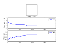
Spontaneous magnetisation^[3] is when the spins take an ordered structure below the curie temperature $T_{c}$ in this case it is likely possible as it does eventually take an ordered state and considering the temperature that ILanim runs at is 0.5 and the theoretical curie temperature is 2.269 it is possible that it would occur but it would take along time/many steps altering the configuration.

Accelerating the code

The script ILtimetrial.py was used to determine the amount of time taken to do 2000 steps of the monte carlo simulation. This was evaluated using IsingLattice.py. The IsingLattice.py code was then optimised through the use of the numpy roll, multiply and sum functions to make the calculation of energy and magnetisation much faster, the results of said optimisation can be seen with the optimised code in fig 5. On average the time decreased by a factor of approximately 4, with the rest of the results remaining the same thus showing it functioned correctly in regards to calculating values just at a much faster speed.

*fig.5* Portion of the code that has been optimised

JC: The energy function is correct and you have used the minimum number of roll operations needed which ensures the code is optimised. However, the magnetisation function has not been optimised as you still have two loops, one over lattice columns and then over lattice rows. The np.sum() function will sum all of the lattice points in one go, without the need for loops and this the optimisation. Your magnetisation function will still give the correct magnetisation, but should operate at a similar speed to the previous magnetisation function, so it has not been optimised.

Unoptimised vs Optimised speeds
run #	Unoptimised/s	Optimised/s
1	11.77575894	3.109330021
2	11.78240738	3.113359185
3	11.82432489	3.11393273
4	11.77386159	3.114423963
5	11.95350621	3.111418797
Mean	11.8219718	3.112492939
Standard deviation	0.076358371	0.002104166
Standard error	0.034148502	0.000941012

JC: Give values to a sensible number of significant figures.

This also resulted in very little error between the runs, 0.034148502 and 0.000941012 for unoptimised and optimised respectively the values calculated are extremely congruent with each other and as such the optimisation can be considered significant.

The effect of temperature

Using ILfinalframe the point of equilibration was chosen as 15000 this can be seen in fig 7 this was confirmed by running it multiple times with varying lattice sizes 8, 16 and 32 all of which provided a very similar result trend wise however as the lattice size increased the steps required to reach equilibrium was also greater and as such a compromise number was chosen of 15000, this was enough to come close to equilibrium for the larger lattices without losing alot of valid data for the smaller ones. These have been omitted as they are very repetitive and thus to be concise only the 16x16 is shown.

*fig 6.* Full MonteCArlo script with adjusted average loop

JC: Well done for noticing that the cut off needed depends on system size. It would be good to plot the larger system, rather than the 16x16 system so that you can show that is has come to equilibrium for your choice of cut off.

The adapted code can be seen in fig 6 the average values have been changed to omit the energy values pre 15000 so an accurate average energy for the system at equilibrium can be established.

JC: You have not taken the cut off into account when you calculate the averages, you need to divide by (self.n_cycles - 15000) in the statistics() function. Also try to number the figures in the order that they are referenced in the text.

Running over a range of temperatures

Using ILtemperaturerange.py the relationship between the energy and temperature as well as magnetisation with temperature was established. As can be seen in fig 8. For the 8x8 lattice the energy showed an overall increase initially very slowly then a slightly steeper increase around the theoretical critical temperature of 2.269² once past the critical region the energy increase returns to its much lower gradient. The overall shape is somewhat reminiscent of $t a n h (x)$ just not through the origin. Regarding magnetisation there is large fluctuation around the critical temperature with the overall magnetisation decreasing significantly, this is to be expected as at the critical/curie temperature the ferromagnet switches from a disordered structure to an ordered one. Note also that the errors are at their largest around the curie temperature for the same reason.

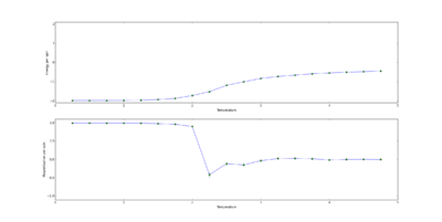
JC: Good observation, if you solve the 2D Ising model using the mean field approximation, you can show that there is a tanh dependence of magnetisation on temperature. It would be good to have a discussion on how the energy and magnetisation changes with temperature in terms of energy and entropy.

Effect of system size

The previous part was then run again using the 2x2, 4x4, 16x16 and 32x32 lattices. The results of these were then loaded on to a single plot, the code for this is in figs 10 and 11, and as can be seen in fig 9 the trends mirror each other in regards to both energy and magnetisation. One thing to note which will be explored later in more detail is the fact that curie temperature actually increases slightly as we increase the lattice size. This can be seen by the shift to higher values of the decrease in magnetisation as well as the overall increase in energy gradient. The largest discrepancy was going from 2x2 to 4x4. The 2x2 lattices seem to be the most temperature sensitive in terms of alternating

configurations as it takes a much lower temperature to force the spins into an ordered state as seen in fig. 11 in which at a temperature less than 1 the magnetisation decreases sharply before plateauing whereas the next largest lattice 4x4 requires a temperature of around 2.2 one possible reason for this is because there are so much less configurations to go through to reach the ordered state that only a small amount of energy si required proportionally to the rest of the lattices. For all the magnetisations there is a large amount of fluctuations about the Curie temperature as to be expected.

For energy the 2x2 once again is very different ending at a much lower energy than the rest of the lattices at the given temperature and as such the energy can be said to be less reliant on temperature than the other lattice sizes due to the decreased gradient. 16x16 seems to be the best to observe long range interactions as its the smallest one that has significant fluctuation but is also big enough to establish a reasonably long range propagation of fluctuation.

JC: Why have you said the 16x16 lattice is better able to observe long range fluctuations than the 8x8 lattice? From your fig. 10 plot the energy curves for 8x8 system and above appear to have converged.

Determining Heat Capacity

The first part of this section of the experiment involved showing that

$C = \frac{\partial ⟨ E ⟩}{\partial T} = \frac{V a r [E]}{k_{B} T^{2}}$

$⟨ E ⟩ = \frac{1}{Z} \sum E (α) e x p [\frac{- E (α)}{k_{B} T}]$

Define $β$ as $\frac{1}{k_{B} T}$

This is the thermodynamic beta.

Define the partition function $Z = \sum e x p [\frac{- E (α)}{k_{B} T}] = \sum e x p [- β E (α)]$

Thus $⟨ E ⟩ = - \frac{1}{Z} \frac{\partial Z}{\partial β}$ where $\frac{\partial Z}{\partial β} = - \sum E (α) e x p [- β E (α)]$

$⟨ E^{2} ⟩ = \frac{1}{Z} \sum E (α)^{2} e x p [- β E (α)]$ = $\frac{1}{Z} \frac{\partial^{2} Z}{\partial β^{2}}$

$V a r [E] = ⟨ E^{2} ⟩ - {⟨ E ⟩}^{2}$

Thus $V a r [E] = \frac{1}{Z} \frac{\partial^{2} Z}{\partial β^{2}} - (- \frac{1}{Z} \frac{\partial Z}{\partial β})^{2}$

Thus $V a r [E] = \frac{\partial^{2} l n Z}{\partial β^{2}}$

This is equal to $- \frac{\partial E}{\partial β} = - \frac{\partial E}{\partial T} \frac{\partial T}{\partial β}$ where $\frac{\partial T}{\partial β} = - k_{b} T^{2}$

Thus $V a r [E] = k_{b} T^{2} \frac{\partial E}{\partial T}$

Therefore $V a r [E] = k_{b} T^{2} C$ and so by rearrangement $C = \frac{V a r [E]}{k_{B} T^{2}}$

JC: Derivation is correct.

The script for evaluating the heat capacity for all of the lattice sizes can be seen in fig 12. The results of this can be seen in figure 13, the results were not what one would expect and while this will be elaborated on later in the report it can be seen that at very low temperatures the heat capacity is abnormally high and while parabolas are present in the lower lattice sizes its hard to isolate them for the bigger sizes.

*fig 12* Script to produce all heat capacities

*fig 13* Heat capacities against temperature for all lattice sizes

Fitting Polynomials

The values for the energies, magnetisation and heat capacities for given lattice sizes were compared to ones computed at very long runtimes and these can be seen in figures 14 to 20. For lattice sizes 2,4 and 8 there was almost no difference in the energies between the computed results and those of the C++ values but at the higher lattice sizes of 16 and 32 there were some very minor discrepancies.

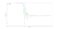
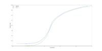
The magnetisation showed significantly more discrepancies not in trend but in regards to fluctuation , while the computed results did fluctuate about the curie temperature the fluctuation was much more significant for the c++ results. For the much longer times it is feasible to predict a much larger fluctuation as longer runtime means more results for a given temperature. Regardless the general trend remains consistent, with the spins forming an ordered state past the curie temperature.

The major discrepancies came with the heat capacity despite having near identical energies the heat capacity values were extremely different with the low temperatures having very high heat capacity for my code as opposed to starting low and forming a parabola, these parabola are observable in my lower lattice size codes but as the lattice size increases rather than forming the parabola my curve starts high and follows the C++ parabola down along a similar gradient but it doesn't increase to a maxima rather starts high and decreases in gradient as the temperature increases. This is obviously a programming error and is most likely to do with the calculation of $E^{2}$ as the energies are near identical and the formula for the heat capacity seems to be correct. This error will be evaluated further in the conclusion. The highest Lattice size with a valid heat capacity curve is seen in fig.20 with 4x4.

JC: You are right that the heat capacity curves are not what you would expect. This may be because you didn't take the cut off into account when you calculate the averages in the statistics function. However, this should also affect the energy that you calculate, but this seems to agree well with the C++ data.

*fig 21* 16x16 Energy as a function of Temperature comparison with C++ script

*fig 23* 4x4 Heat Capacity as a function of temperature comparison with C++ script

*fig 24* Script to fit polynomials to the curves, in this case it is for C++ data. Note this also contains lines that fit it in a particular temperature range.

A polynomial was then fit to the curves as can be seen in figures 25,26 and 27. figures 25 and 27 show curves fit to the 4x4 created by my code and the C++ code respectively, this is because for the heat capacity the parabola for my code wasn't as defined for lattice sizes greater than 4x4 and as such its hard to compare them to the C++ code, for my code the order of polynomial required for an accurate fit was 9 and for the C++ code the required order was 7. Fitting the polynomial is extremely useful as it allows for analysis of things like maximum peaks in data as well as determining uncertainty. For my curve due to it's lack of major fluctuation is showed an exceptional fit to the polynomial with barely any discrepancy and thus can be considered useful and accurate to the general trend. The polynomial was chosen to be fit between T values of 1 and 4 to remove as much of the discrepancies as possible in the anomalous Heat capacity data. The script for this can be seen in fig 24

The final part involved finding the peak in C, the issue with doing so is because my parabolas aren't apparent for higher lattice sizes there isn't a distinguishable peak and as such rather than doing it for my actual data, in order to approximate where the peak in C would be as the gradient seemed to be relatively indicative of where the parabola would be if the lower temperature values weren't anomalous and since the polynomials were able to fit in a manner that was near identical to the parabolas in 2x2 and 4x4 as well as curving the expected way for larger lattice sizes, rather than coding to get my max Temperature value from my values I though it would be best to attempt to approximate based on the fitted values of the polynomials as these would be roughly what I would've gotten if the values hadn't been incorrect for the lower temperatures. Note that the lower limit when considering my data is 1.25 to start at a point past the anomalous data for the smaller lattices which show the parabola, this is relatively useless in the case of higher lattice sizes as since they show a purely negative gradient the highest value would always be Tmin regardless. This is also applicable because there is a very minor positive gradient towards the peaks of the 'parabolas' at higher lattice sizes which can be somehwat isolated with the polynomial fit but once again the values are going to have very large errors due to being approximations.

*fig 28* Script for Determining Tmax for the fitted values

*fig 29* Script to plot Tmax as a function of lattice size

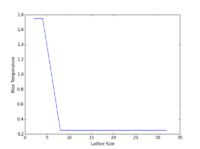
The code used for these processes can be seen in figs 28 and 29. This lead to 2x2 and 4x4 giving a maximum temperature of 1.75 and 2.5 for the larger sizes suggesting a value between this for the Curie temperature, the theoretical temperature as mentioned previously is 2.269 which lies between these values so the approximation while somewhat rudimentary still gives a 'ballpark' range for the value.

JC: Without understanding where the heat capacity calculation has gone wrong and correcting it it is very difficult to predict the Curie temperature. What does fig. 30 show, did you use this to calculate the heat capacity?

Conclusion

This experiment as a whole was a success, aside from the heat capacity all of the rest of the data produced via the simulations i.e. the magnetisation and energy for give lattice sizes were determined and were relatively close to the theoretical values. There were very few errors in trends as well as strong congruency with the C++ data suggesting that for the most part the results were accurate.

The obvious large error comes in the heat capacity, the anomaly is strange in the sense that at lower lattice sizes the maxima are still visible but as the size increased the curve changes into a negative gradient sloping down from a high value at lower temperatures to very low values at higher temperatures. Interestingly the graphs seemed to follow almost the same gradient as the negative gradient slope of the expected maxima as shown when comparing to the C++ data. The most likely point of error for this is in the running total of energysq as the energies were the same/similar for both my data sets and the C++ and the formula for heat capacity seemed to be computed correctly thus leaving that as the most likely option. Unfortunately to remedy this the only would've been to restart from near the beginning of the experiment which due to how long computing the larger lattice sizes thermodynamic properties took just wasn't feasible in the time remaining. As such to make sure the data wasn't wasted an polynomial was fit to the data and due to the nature of it following the same gradient as well as having a very minor peak mimicking the expected maxima it was possible to get, albeit a very rough one, an approximation of the requested values. Ideally without a time limit on the assignment this could've been remedied from the beginning so this wouldn't be necessary however with the options available this was arguably the only possible one for the circumstances.

References

1. Taken from Imperial chemistry Third year CMP compulsary experiment lab script https://wiki.ch.ic.ac.uk/wiki/index.php?title=Third_year_CMP_compulsory_experiment/Introduction_to_Monte_Carlo_simulation

2. David P. Landau, K. K. Mon, H. B. Schüttler. Computer Simulation Studies in Condensed-Matter Physics IX. : Springer Verlag Berlin Heidelberg; 1997.

3. Barry M. Mccoy, Tai Tsun Wu. The Two-Dimensional Ising Model, 2nd ed. Mineola New York: Dover Publications Inc; 2014.