
Talk:MIKE123
JC: General comments: All tasks answered and data looks good. Try to make your explanations of your results clearer and more focused and bring in some of the background theory where appropriate to show your understanding.
Transition States and Reactivity
Introduction to the Icing Model
The Model
Task 1: Lowest Energy of the Icing model
The interaction energy is defined as , where the first sum loops over the number of spins in the system and the second sum loops over the number of neighbours. When keeping all parameters constant apart from the number of dimensions, the only thing changing is the second sum.
For the number of neighbours is , for it's and for it's . In general one can say that it the number of neighbours is .
In the lowest energy state all spins will be aligned leading to maximum multiplicity and thus a scenario where for all and. As the value of can only have the values or , the product under the sum must always equal to .
This interaction energy equation therefore simplifies to . The cancels out with the from and once the sums are evaluated they simplify to . q.e.d.
The entropy of this system is given by , where is the multiplicity. In this system the multiplicity is one as there is only one configuration for a particular state when all spins are aligned. Thus the entropy equals to zero.
JC: Correct. Did you consider that the ground state can be all spin up or all spin down?
Phase Transitions
Task 2: Energy change caused by a change in state and the entropy involved
Using the equation for the interaction energy for the lowest state from above, the lowest energy configuration has a value of . In order to obtain an energy for the system when one spin is antiparallel to the others one can examine the general equation. The antiparallel spin will occur as once and as 6 times (for 6 different neighbours once). This will lead to terms adding to the energy and terms cancelling out each other eventually leading to a value of . So the energy change is .
JC: Can you show more of the maths working for this step.
The flipping of the spin can happen on any point of the 1000 sites in the lattice. This demonstrates that there are 1000 configurations where one spin is antiparallel to the others. This leads to an entropy value gain of
JC: Correct.
Task 3: Magnetisation in a 3-D lattice
As there is always one more positive spin in both the 1D and 2D lattice, both systems have a magnetisation of .
Absolute zero indicates that all spins in a system are aligned, so they either all have an value of or , leading to a total magnetisation of either or respectively.
Calculating the energy and magnetisation
Task 4: completing the energy() and magnetisation() function
Please refer to the comments in the code:
    def energy(self):
        energy = 0.0
#copying the boundaries of the lattice and extending/appending them on the opposite ends in all four directions
        new_lattice = np.append(self.lattice, [self.lattice[0]], axis=0)
        new_lattice2 = np.append([self.lattice[-1]], new_lattice, axis = 0)
        new_lattice3 = np.concatenate((np.transpose([new_lattice2[:,-1]]),new_lattice2), axis = 1)
        new_lattice4 = np.concatenate((new_lattice3, np.transpose([new_lattice3[:,1]])), axis = 1)
#looping through the new lattice
        for ycor in range(len(new_lattice4)):
            for xcor in range(len(new_lattice4)):
#this makes sure that only the points from the original lattice are counted
                if ycor >0 and ycor < len(new_lattice4)-1 and xcor >0 and xcor < len(new_lattice4[0])-1:
#checks the energy in every direction and adds the contribution
                    if new_lattice4[ycor][xcor] + new_lattice4[ycor-1][xcor] == 0:
                        energy += +0.5
                    else:
                        energy += -0.5
                    if new_lattice4[ycor][xcor] + new_lattice4[ycor+1][xcor] == 0:
                        energy += +0.5
                    else:
                        energy += -0.5
                    if new_lattice4[ycor][xcor] + new_lattice4[ycor][xcor-1] == 0:
                        energy += +0.5
                    else:
                        energy += -0.5
                    if new_lattice4[ycor][xcor] + new_lattice4[ycor][xcor+1] == 0:
                        energy += +0.5
                    else:
                        energy += -0.5
        return energy

    def magnetisation(self):
#sum() was assumed common knowledge
        magnetisation = np.sum(self.lattice)
        return magnetisation
JC: Code looks good and is well commented.
Task 5: Checking the code using the ILcheck.py script
The values seemed to match!

Introduction to the Monte Carlo simulation
Average Energies and Magnetisation
Task 6: Configuration of 100 spins and the estimated time it takes to evaluate the average magnetisation at one temperature
In a system of 100 spins there are configurations. In base 10 this approximates to about configurations. So dividing this number by the computational rate of configurations per seconds gives us a time of seconds or about years.
JC: So evaluating every configuration is not possible.
Modifying IsingLattice.py
Task 7: Completing the montecarlostep function and the statistics function to obtain values for and
Please refer to the comments in the code below:
    def montecarlostep(self, T):
#saving the energy before the change
        energy0 = self.energy()
        magnet0 = self.magnetisation()
#the following two lines will select the coordinates of the random spin for you
        random_i = np.random.choice(range(0, self.n_rows))
        random_j = np.random.choice(range(0, self.n_cols))
#flipping the spins in the original lattice
        if self.lattice[random_i][random_j] == -1:
            self.lattice[random_i][random_j] += 2
        else:
            self.lattice[random_i][random_j] -= 2
#saving the energy after the change
        energy1 = self.energy()
        magnet1 = self.magnetisation()
        energy_d = energy1 - energy0
#the following line will choose a random number in the range [0,1) for you
        random_number = np.random.random()
#checking whether the original lattice should have been kept (rather than checking if we should change)
        if energy_d > 0 and random_number > np.e**(-energy_d/T):
#if yes then the spin is flipped back and the original energy is stored in energy1
            if self.lattice[random_i][random_j] == -1:
                self.lattice[random_i][random_j] += 2
            else:
                self.lattice[random_i][random_j] -= 2
            energy1 = energy0
            magnet1 = magnet0
#always append the energy1 from the new system/corrected-back system
        self.E += energy1
        self.E2 += energy1**2
        self.M += magnet1
        self.M2 += magnet1**2
        self.n_cycles += 1
        return energy1, magnet1

    def statistics(self):
#divide by cycles, have an if condition so that it doesn't crash when n_cycles = 0
        if self.n_cycles > 0:
            avg_e = self.E/self.n_cycles
            avg_e2 = self.E2/self.n_cycles
            avg_m = self.M/self.n_cycles
            avg_m2 = self.M2/self.n_cycles
            return avg_e, avg_e2, avg_m, avg_m2, self.n_cycles
        else:
            return self.E, self.E2, self.M, self.M2, self.n_cycles
JC: Looks correct, to flip the spin you could just multiply the spin by -1.
Task 8: Discussing the the behaviour of a system when
As given in the instructions, the system under investigation is set to be below the , so that is fulfilled. In this case thermal energy is too low to influence any entropic forces, so that it is very unlikely that higher spin energy states are populated spontaneously. Thus what will happen is that the system tries to minimise it's energy by aligning all spins. This will lead to all spins being parallel and thus . This was also observed when running ILanim.py on the system:

| Quantity after 445 steps | Value after 445 steps |
|---|---|
| -1.329485 | |
| 2.120480 | |
| 0.664477 | |
| 0.536613 |
Accelerating the code
Task 9: Duration of ILtimetrial.py for 2000 Monte Carlo steps
Duration for 2000 Monte Carlo Steps:
| Trial | Time (s) |
|---|---|
| 1 | 17.46 |
| 2 | 17.55 |
| 3 | 17.52 |
So one can safely assume the code executes within about 17.5 +/- 0.2 seconds.
Task 10: Improving the energy() and magnetisation() function
    def energy(self):
        energy = 0.0
        s_ilattice = self.lattice
#creates four lattices which are shifted with respect to s_ilattice in the four directions by one item (they wrap around edges)
        s_jlattice1 = np.roll(s_ilattice, 1, axis=0) #down
        s_jlattice2 = np.roll(s_ilattice, -1, axis=0) #up
        s_jlattice3 = np.roll(s_ilattice, 1, axis=1) #right
        s_jlattice4 = np.roll(s_ilattice, -1, axis=1) #left
#they are added essentially creating a latticesum of neighbours for every item in s_ilattice
        s_jlatticesum = s_jlattice1 + s_jlattice2 + s_jlattice3 + s_jlattice4
#the coordinates of an item in s_ilattice correspond to the coordinates of the sum of its neighbours in s_jlatticesum
#multiplying them with each other gives s_i *s_j for all neighbours
#taking the sum in order to get a total energy throughout the lattice
        energy += np.sum(np.multiply(s_ilattice, s_jlatticesum))*(-0.5)
        return energy

#as before
    def magnetisation(self):
        magnetisation = np.sum(self.lattice)
        return magnetisation
JC: You actually only need to use roll twice (if you remove the factor of 0.5 from the energy) as this prevents double counting of interactions.
Task 11: Duration of ILtimetrial.py for 2000 Monte Carlo steps after function improvement
| Trial | Time before improvement (s) | Time after improvement (s) |
|---|---|---|
| 1 | 17.46 | 0.42 |
| 2 | 17.55 | 0.43 |
| 3 | 17.52 | 0.43 |
Thus an average of about 0.43 +/- 0.1 seconds for the 2000 Monte Carlo Steps can be assumed. This is a major improvement of about 17 seconds. A major contributor to this improvement in run time is certainly the removal of for loops and the implementation of built in functions.
The effect of temperature
Correcting the Averaging Code
Task 12: Adjusting the code to account only for fluctuations around the equilibrium state
# global variable has been implemented which can be altered at wish
    ignored_cyc = 225000

    def montecarlostep(self, T):
        energy0 = self.energy()
        magnet0 = self.magnetisation()
        random_i = np.random.choice(range(0, self.n_rows))
        random_j = np.random.choice(range(0, self.n_cols))
        if self.lattice[random_i][random_j] == -1:
            self.lattice[random_i][random_j] += 2
        else:
            self.lattice[random_i][random_j] -= 2
        energy1 = self.energy()
        magnet1 = self.magnetisation()
        energy_d = energy1 - energy0
        random_number = np.random.random()
        if energy_d > 0 and random_number > np.e**(-energy_d/T):
            if self.lattice[random_i][random_j] == -1:
                self.lattice[random_i][random_j] += 2
            else:
                self.lattice[random_i][random_j] -= 2
            energy1 = energy0
            magnet1 = magnet0
#energies are only added if the number of cycles is larger than the number of ignored cycles
        if self.n_cycles > self.ignored_cyc:
            self.E += energy1
            self.E2 += energy1**2
            self.M += magnet1
            self.M2 += magnet1**2
        self.n_cycles += 1
        return energy1, magnet1

    def statistics(self):
        if self.n_cycles > 0:
#statistical values are calculated with the corrected number of cycles
            avg_cycles = self.n_cycles - self.ignored_cyc
            avg_e = self.E/avg_cycles
            avg_e2 = self.E2/avg_cycles
            avg_m = self.M/avg_cycles
            avg_m2 = self.M2/avg_cycles
            return avg_e, avg_e2, avg_m, avg_m2
        else:
            return self.E, self.E2, self.M, self.M2
The system was analysed for a grid of and at temperatures of and . It was discovered that as the critical temperature lies somewhere between those two temperatures, as below the system took time (up to 225000 steps) to reach equilibrium while when the system had enough thermal energy to easily overcome the energy barrier and thus reach equilibrium really fast (less than 1000 steps) . The latter observation is due to the fact that a above the Curie Temperature random magnetisation is very unlikely to happen. It was further observed that at bigger lattice sizes the time it took for the system to reach equilibrium was larger. It was thus concluded that in order to be prepared for the worst case scenario ( with just under ), a total of 225000 cycles will be ignored. This number can be obtained from observing the last graph.
-
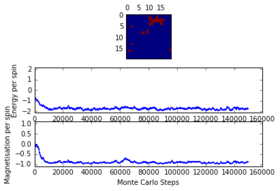 16x16 at T = 2.0, 150000 steps
 -
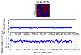 16x16 at T = 4.0, 150000 steps
 -
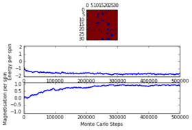 32x32 at T = 2.0, 500000 steps
 -
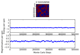 32x32 at T = 4.0, 500000 steps


JC: Good analysis and correctly implemented in code.
Running over a range of temperatures
Task 13: Average Energy and Magnetisation for each Temperature
It was decided that the simulations will run in the temperature range ofand in steps of for a total number of 350000 steps with 225000 steps being disregarded in the energy and magnetisation averages. The results are presented in the next section.
The effect of system size
Scaling the System Size
Task 14: Energy per spin versus temperature diagrams for different lattice sizes
In order to plot the functions from the obtained data files the following function was defined to be called for every lattice size and the output is shown below.
import numpy as np
from matplotlib import pylab as plt


def plotfunct(filename, lattice_side_size):
    data = np.loadtxt(filename)
    temps = data[:,0]
    energies=data[:,1]
    energies2=data[:,2]
    magnet=data[:,3]
    magnet2=data[:,4]
    spins = lattice_side_size**2
#errorbars as square root of variance, energies are given per spin
    energies_error = np.sqrt(energies2-energies**2)/spins
    magnet_error = np.sqrt(magnet2-magnet**2)/spins

    plt.ylabel("Energy per spin")
    plt.xlabel("Temperature")
    plt.title('Energy per spin vs Temperature (' + str(lattice_side_size)+'x'+str(lattice_side_size)+')')
    plt.errorbar(temps, energies/spins,yerr = energies_error, ecolor = "green")
    plt.show()
    plt.ylabel("Magnetisation per spin")
    plt.xlabel("Temperature")
    plt.title('Magnetisation per spin vs Temperature (' + str(lattice_side_size)+'x'+str(lattice_side_size)+')')
    plt.errorbar(temps, magnet/spins, yerr = magnet_error, ecolor = "green")
    pl.show()
As lattice size increases, fluctuations and error bars decrease massively. It is further observed that the point at which equilibrium is reached in the magnetisation graph shifts from left to right (to increasing temperature) as lattice size is increasing. The first observation can be explained through the way data is processed. In small systems like 2x2, flipping of one spin has a huge impact on the absolute change in energy (1 in 4 spins), whereas the same flip in a 32x32 system has a minor contribution (1 in 1024). Latter will thus have a much smaller impact on the statistical means that are used to obtain the graphs. The second observation can also be explained through the quantity of spins in each lattice. As the Monte Carlo algorithm assigns multiple random numbers when it is called, it is much more likely to totally reverse a small system than a large one. I.e. completely reversing a system is much more likely to happen in a 2x2 lattice (4 different flips needed) versus a 32x32 lattice (1024 different flips needed!!!).
The quality of the data (reduced noise) does not seem to linearly depend on lattice size (judged by eye). However it does definitely increase with increasing lattice size. While 32x32 seems adequate to perform calculations with, 64x64 would very likely improve the data even more.


JC: Graphs look good, did you also plot the energy per spin for each system size on the same axes to compare them?
Determining the heat capacity
Calculating the heat Capacity
Task 15: Deriving an expression for heat capacity from the partial derivative expression
1. The heat capacity is given as , with
2. Defining and for simplification purposes and noting that
3. The expression which should be derived is , where .
4. So from that an expression for and in terms of and shall be found.
5. Differentiating with respect to gives: .
6. Using this information can be rewritten as
7. Differentiating with respect to twice gives:
8. Thus can be rewritten as
9. Evaluating the original expression using the product rule gives:
10. Applying the chain rule twice in the first term and once in the second term gives:
11. Substituting the expressions for the partial derivatives from 2., 6. and 8., hence gives:
JC: Derivation is correct, but it might be easier to follow if you can just start from one side of the equation and show the steps needed to reach the other side.
Task 16: Plotting Heat Capacity vs Temperature for different lattice sizes
import numpy as np
from matplotlib import pylab as plt


def plotheatcap(filename, lattice_side_size):
    data = np.loadtxt(filename)
    temps = data[:,0]
    spins = lattice_side_size**2
    energies=data[:,1]
    energies2=data[:,2]
    varian = (energies2-energies**2)/spins

    plt.ylabel("Heat Capacity")
    plt.xlabel("Temperature")
    plt.plot(temps, varian/temps**2, label = str(lattice_side_size) + "x"+ str(lattice_side_size))


def plotmultiple(filenamearray, lattice_side_array):
    for i in range(len(filenamearray)):
        plotheatcap(filenamearray[i], lattice_side_array[i])
    plt.title("Heat capactiy per spin vs temperature for various lattice sizes")
    plt.legend(loc="best",title="Lattice size",fontsize="8")
    plt.show()

plotmultiple(['2x2.dat','4x4.dat','8x8.dat','16x16.dat','32x32.dat'],[2,4,8,16,32])
This code leads to the graph below. The heat capacity per spin seem to slightly increase with the size of the lattice. The peak does also seem to become more narrow. This directly relates to the previous discussion about lattice size affecting statistical measures, as heat capacity is directly related to the variance of the obtained energies. I.e. larger spins system lead to smaller error / variance and thus a more narrow peak of the heat capacity. Ideally at very large lattice size this peak will become as narrow as possible.
JC: For an infinite lattice the peak diverges.

Locating the Curie temperature
C++
Task 17: Comparing the quality of data obtained using python versus C++
import numpy as np
from matplotlib import pylab as plt


def plottwocap(filenamearray, lattice_side_array):
    plotheatcap(filenamearray[0],lattice_side_array[0])

    data2 = np.loadtxt(filenamearray[1])
    temps2 = data2[:,0]
    spins2 = lattice_side_array[1]**2
    energies2=data2[:,1]
    energies22=data2[:,2]
    varian2 = (energies22-energies2**2)
    capa = data2[:,5]

    plt.ylabel("Heat Capacity")
    plt.xlabel("Temperature")
    plt.plot(temps2, capa, label = "C++")
    plt.title("Heat capactiy per spin vs temperature (32x32)")
    plt.legend(loc="best",title="Lattice size",fontsize="8")
    plt.show()

def plottwo2(filenamearray, lattice_side_array):
    data1 = np.loadtxt(filenamearray[0])
    temps1 = data1[:,0]
    spins1 = lattice_side_array[0]**2
    energies = data1[:,1]
    magnet = data1[:,3]

    data2 = np.loadtxt(filenamearray[1])
    temps2 = data2[:,0]
    energies2=data2[:,1]
    magnet2 = data2[:,3]

    plt.ylabel("Energy per spin")
    plt.xlabel("Temperature")
    plt.title('Energy per spin vs Temperature (' + str(lattice_side_array[0])+'x'+str(lattice_side_array[0])+')')
    plt.plot(temps1, energies/spins1,label="python")
    plt.plot(temps2, energies2,label="C++")
    plt.legend(loc="best",title="Language",fontsize="8")
    plt.show()

    plt.ylabel("Magnetisation per spin")
    plt.xlabel("Temperature")
    plt.title('Magnetisation per spin vs Temperature (' + str(lattice_side_array[0])+'x'+str(lattice_side_array[0])+')')
    plt.plot(temps1, magnet/spins1,label="python")
    plt.plot(temps2, magnet2,label="C++")
    plt.legend(loc="best",title="Language",fontsize="8")
    plt.show()

plottwo2(['32x32.dat','C++_data/32x32C.dat'],[32,32])

plottwocap(['32x32.dat','C++_data/32x32C.dat'],[32,32])
The data from the C++ files was collected in steps of rather than as was done in the previous section. This lead to a higher data rate and higher resolution in all graphs. It was especially noticeable in the region around the Curie Temperature for the magnetisation per spin graph as fluctuations were made visible which were originally assumed completely absent.


Polynomial fitting
Task 18: Polyfitting Heat Capacity to a polynomial
import numpy as np
from matplotlib import pylab as plt

def plotpolyfit(filename):
    dataA = np.loadtxt(filename)
    temps = dataA[:,0]
    capa = dataA[:,5]

    fit = np.polyfit(temps,capa,5)
    fit2 = np.polyfit(temps,capa,100)
    T_min=np.min(temps)
    T_max=np.max(temps)
    T_range=np.linspace(T_min,T_max,1000)
    fitted_C_values = np.polyval(fit,T_range)
    fitted_C_values2 = np.polyval(fit2,T_range)

    plt.plot(temps,capa,label='Collected Data')
    plt.plot(T_range,fitted_C_values,label='Fitted Data (Degree 5)')
    plt.plot(T_range,fitted_C_values2,label='Fitted Data (Degree 100)')
    plt.legend(loc ="best", fontsize= 8)
    plt.title('Heat Capacity per Spin Curve Fitting (32x32)')
    plt.xlabel('Temperature')
    plt.ylabel("Heat Capacity")
    plt.show()

plotpolyfit('C++_data/32x32C.dat')
Some initial trials to polyfit a polynomial to the whole data range only showed little success. Even when increasing the polynomial degree to 100, it was not possible to approximate the peak accurately.

Task 19: Polyfit the heat capacity to a polynomial in a specific temperature range
import numpy as np
from matplotlib import pylab as plt

def plotpolyfitinrange(filename, dimension, minT, maxT, degree):
    dataA = np.loadtxt(filename)
    temps = dataA[:,0]
    capa = dataA[:,5]

    selection = np.logical_and(temps > minT, temps < maxT) #choose only those rows where both conditions are true
    peak_T_values = temps[selection]
    peak_C_values = capa[selection]

    fit = np.polyfit(peak_T_values,peak_C_values,degree)
    T_min=np.min(temps)
    T_max=np.max(temps)
    T_range=np.linspace(T_min,T_max,1000)
    fitted_C_values = np.polyval(fit,T_range)
    fitted_C_values2 = np.polyval(fit,peak_T_values)
    Cmax = np.max(fitted_C_values2)
    Tmax = peak_T_values[fitted_C_values2 == Cmax]
    print(Cmax, Tmax)
    plt.plot(temps,capa,label='Collected Data')
    plt.plot(T_range,fitted_C_values,label='Fitted Data between ['+ str(minT) +','+str(maxT)+'] (Degree '+str(degree)+')')
    plt.legend(loc ="best", fontsize= 8)
    plt.title('Heat Capacity per Spin Curve Fitting (' + str(dimension)+'x'+str(dimension)+')')
    plt.xlabel('Temperature')
    plt.ylabel("Heat Capacity")
    plt.ylim([-0.5,2])
    plt.show()

plotpolyfitinrange('C++_data/2x2C.dat',2,1.5,3.4,4)
plotpolyfitinrange('C++_data/4x4C.dat',4,1.5,3.4,4)
plotpolyfitinrange('C++_data/8x8C.dat',8,1.7,3,6)
plotpolyfitinrange('C++_data/16x16C.dat',16,2,2.7,6)
plotpolyfitinrange('C++_data/32x32C.dat',32,2.2,2.4,5)
A big improvement was made when small regions were selected to run through the polyfit function. The last parameter in the function "plotpolyfztinrange" above indicates the polynomial degree used for further calculations. By reducing the domain of the function, even polynomial of degree 4 were enough to accurately fit the heat capacity data (for 2z2 and 4x4).

JC: Fit looks good.
Task 20: Plotting the scaling relation between the Curie Temperature and the lattice side length
The data for the table below was obtained when executing the previous function for every lattice. It showed that the Curie Temperature decreased with increasing lattice size as was expected in the provided function of .
| Size | Temperature |
|---|---|
| 2x2 | 2.52 |
| 4x4 | 2.48 |
| 8x8 | 2.36 |
| 16x16 | 2.32 |
| 32x32 | 2.30 |
In order to obtain the Currier temperature at infinite lattice the temperatures (table above) at which the heat capacities were maximised were plotted against the inverse of the respective lattice side length, .
from matplotlib import pylab as plt
import numpy as np

sidelength = np.array([2,4,8,16,32])
curieT = np.array([2.52,2.48,2.36,2.32,2.30])

fit = np.polyfit(1/sidelength, curieT, 1, cov=True)
params = fit[0]
params_cov = fit[1]

x_range = np.linspace(0, 0.5, 1000)
fitted_curie = params[0]*x_range + params[1]
plt.xlabel("1/L")
plt.ylabel("Curie temperature")
plt.plot(1/sidelength, curieT, linestyle='',marker='x',label="Collected Data")
plt.plot(x_range, fitted_curie, label="Linear fit")
plt.title("Curie temperature versus 1/L for LxL lattices")
plt.legend(loc="best",fontsize=10)
plt.show()

A value of for the Currier Temperature at infinite lattice was obtained (y-intercept). This result lies within the boundaries of the literature value of 2.269.[1]. However, when analysing the graph below it seems quite obvious that the point at 2x2 is an outlier. The reasons for that were discussed thoroughly in previous sections above as the uncertainty of the 2x2 lattice's data continuously showed up throughout this report.
Additional minor factors that contribute to this deviation from the literature value will come from the method used, i.e. the Monte Carlo algorithm rejects complete randomness and is thus an approximation. However, it is actually rather a personal surprise that such a good close result was obtained using this algorithm, that cut down run time from about years to just around 30 minutes. So essentially having a fairly big lattice size of about should be ideal to increase accuracy while sacrificing little additional computational time.
JC: Considering the problems with the 2x2 system, you could remove this data point from the fit and see if it improves the agreement with the theoretical value from the literature.
References
- ↑ L. Onsager, Crystal Statistics. I. A Two-Dimensional Model with an Order-Disorder Transition, Physical Review, 1944, 65, 117-149.