Talk:LiquidSimulationsSL7514

General comments: Very detailed and expansive. Ensure that extension doesn't get in the way of good physics. Think simple and expand but good report. 87/100

Introduction to Molecular Dynamics Simulations

TASK 1

Figure 1. Comparison of position, total energy and error between Harmonic Oscillator solution and Verlet Algorithm for 0.2 timestep, φ=0 and k=m=A=ω=1

TASK 2

Figure 2. Plot of maximum error for each harmonic oscillation where the error was calculated by finding the difference between the Harmonic Oscillator and Verlet Algorithm solutions for 0.1 timestep, φ=0 and k=m=A=ω=1

TASK 3

The total energy of a simple harmonic oscillator is given by:

$E_{tot}=\frac{1}{2}k{x}^2+\frac{1}{2}m{v}^2$

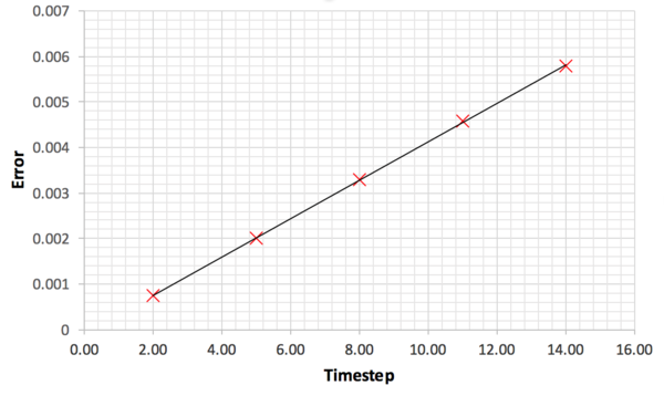
Couple of deductions can be made from Figure 1 and 2. Firstly, the total energy of the system oscillated over the timestep, and the amplitude of the oscillation was more severe when the timestep was larger. When the total energy was equal to 0.5, less than 1% deviation would mean that the total energy must fall within the range 0.5±0.005. As it can be seen from Figure 1, the total energy did not deviate beyond 0.495 when the timestep was set to 0.2. When the position of the particle was either 1 or -1, no deviation in total energy from 0.5 was observed whereas the deviation was greatest when the position of the particle was at 0 or when the velocity of the particle was maximum. The main approximation in velocity-Verlet algorithm was that Taylor expansion of the velocity by half a step was taken. Tick

$v_i(t+\frac{1}{2}\delta t)=v_i(t)+\frac{1}{2}{a}_i(t)\delta t$

Since the expansion was only performed up to the first order term (corresponding to acceleration), the validity of the approximated velocity would be low for large timesteps. Don't think of this as an expansion: the expansion of the Velocity-Verlet comes in the Taylor expansion of x(t + δτ). In order to calculate the new velocity, we take the original velocity and add the velocity change over an average of the change in velocity with time (acceleration). True, this would become increasingly worse for larger timesteps because we would need to numerically calculate the integral Therefore, larger the velocity of the particle, greater the error and hence the maximum from the error plot were observed when the displacement of the particle corresponded to 0. The errors were small at positions corresponding to 1 and -1 because the error in velocity was small as the velocity was close to zero. Since the position was calculated using this calculated velocity, this corresponded to smaller error in position. It should also be noted that the maximum error increased after each cycle due to the propagation in error. If the velocity was calculated incorrectly in the previous cycle, this value was not ignored in the subsequent cycle and hence the error accumulated in the algorithm.

Newtons equations strictly conserve the total energy of the system and hence this should ideally be preserved in the numerical solutions. Monitoring the total energy of the system is important to ensure that the timestep chosen in the simulation is sensible.Tick, but not just timestep - whether fundamentally the system has equilibrated It crucial to remember that in velocity-Verlet algorithm, the simulation has been discretised and hence for large timesteps the Taylor expansion would be inaccurate as only limited number of terms are considered. If the previous configuration is inaccurate, the subsequent coordinates of the atoms or molecules are even more unrealistic and so the energy may not converge to a value but diverge. Unlike the Monte Carlo method, no configurations are ignored in Molecular Dynamics (MD) and the divergence may arise due to the accumulation of error.

Figure 3. Due to the discrete nature of velocity-Verlet algorithm, larger timestep would mean the subsequent configuration of atoms or molecules would be even more unrealistic, leading to propagation of error

TASK 4

At $r_0$, the potential energy must be zero:

$\varphi (r)=4ϵ(\frac{{\sigma }^{12}}{r^{12}}-\frac{{\sigma }^6}{r^6})=0$

$\frac{{\sigma }^2}{r_0^{12}}-\frac{{\sigma }^6}{r_0^6}=0$

$r_0^6={\sigma }^6$

$r_0=|\sigma |$ Tick

The derivative of the Lennard Jones potential is given by:

${\varphi }^{\prime }=4ϵ(-\frac{12{\sigma }^{12}}{r^{13}}+\frac{6{\sigma }^6}{r^7})$

and since the force is given by:

$F=-\frac{d\varphi (r)}{dr}$

when $r=r_0$, the force is given by:

$F=-4ϵ(-\frac{12{\sigma }^{12}}{{\sigma }^{13}}+\frac{6{\sigma }^6}{{\sigma }^7})$

$F=\frac{24ϵ}{\sigma }$ Tick

At the equilibrium, the gradient of the potential must equal zero

${\varphi }^{\prime }=4ϵ(-\frac{12{\sigma }^{12}}{r_{eq}^{13}}+\frac{6{\sigma }^6}{r_{eq}^7})=0$

$\frac{12{\sigma }^{12}}{r_{eq}^{13}}=\frac{6{\sigma }^6}{r_{eq}^7}$

$r_{eq}^6=2{\sigma }^6$

$r_{eq}=2^{\frac{1}{6}}\sigma$Tick

The well depth is given by:

$\varphi (r_{eq})=4ϵ(\frac{{\sigma }^{12}}{r_{eq}^{12}}-\frac{{\sigma }^6}{r_{eq}^6})$

$\varphi (r_{eq})=4ϵ(\frac{{\sigma }^{12}}{4{\sigma }^{12}}-\frac{{\sigma }^6}{2{\sigma }^6})$

$\varphi (r_{eq})=4ϵ(\frac{1}{4}-\frac{1}{2})$

$\varphi (r_{eq})=-ϵ$Tick

The following integrals were evaluated:

$\underset{2\sigma }{\overset{\mathrm{\infty }}{\int }}\varphi (r)dr={[-\frac{4r^{-11}}{11}+\frac{4r^{-5}}{5}]}_{2\sigma }^{\mathrm{\infty }}$

$=[\frac{4}{11}\frac{1}{2^{11}{\sigma }^{11}}-\frac{4}{5}\frac{1}{2^5{\sigma }^5}]=-0.024822$Tick

$\underset{2.5\sigma }{\overset{\mathrm{\infty }}{\int }}\varphi (r)dr={[-\frac{4r^{-11}}{11}+\frac{4r^{-5}}{5}]}_{2.5\sigma }^{\mathrm{\infty }}$

$=[\frac{4}{11}\frac{1}{2.5^{11}{\sigma }^{11}}-\frac{4}{5}\frac{1}{2.5^5{\sigma }^5}]=-0.0081767$Tick

$\underset{3\sigma }{\overset{\mathrm{\infty }}{\int }}\varphi (r)dr={[-\frac{4r^{-11}}{11}+\frac{4r^{-5}}{5}]}_{3\sigma }^{\mathrm{\infty }}$

$=[\frac{4}{11}\frac{1}{3^{11}{\sigma }^{11}}-\frac{4}{5}\frac{1}{3^5{\sigma }^5}]=-0.00329013$Tick

The evaluation of the integrals showed that the potential beyond $3\sigma$ separation of atoms was negligible. In LAMMPS simulations, the potential for each atom was defined within the cutoff distance and hence there were no interaction between atoms with separation greater than this value.

$\varphi (r)=\{\begin{array}{ll}4ϵ(\frac{{\sigma }^{12}}{r^{12}}-\frac{{\sigma }^6}{r^6})& r⩽r_c\\ 0& r>r_c\end{array}$ where $r_c$ is the cutoff distance.Tick

TASK 5

The number of molecules in 1 ml of water was calculated in standard conditions as below. The density of water at standard conditions is one, and hence the number of moles of water in 1 ml is given by:

$$\begin{gathered} mols=\frac{1[g]}{18[g/mol]}=0.0555 \\ mol \end{gathered}$$

$$\begin{gathered} no. \\ of \\ atoms=0.0555\times N_A=3.3456\times 10^{22}atoms \end{gathered}$$Tick

To find the volume of 10000 water molecules at standard conditions, the number of moles of water was calculated first.

$mols=\frac{10000}{6.02214\times 10^{23}}=1.66\times 10^{-20}mols$

$mass=1.66\times 10^{-20}[mols]\times 18[g/mol]=2.99\times 10^{-19}g$

Since the density of water is 1 g/ml, the volume is

$2.99\times 10^{-19}g\times \frac{1}{1[g/ml]}=2.99\times 10^{-19}ml$Tick

TASK 6

When the atom moves from $(0.5,0.5,0.5)$ by $(0.7,0.6,0.2)$, the new position is given by:

$r_{new}=\left(\begin{array}{c}0.5\\ 0.5\\ 0.5\end{array}\right)+\left(\begin{array}{c}0.7\\ 0.6\\ 0.2\end{array}\right)=\left(\begin{array}{c}1.2\\ 1.1\\ 0.7\end{array}\right)$Tick

to take the periodic boundary condition (PBC) into account, whenever the position vector exceeds the unit cell length $(1,1,1)$, this should be subtracted

$r_{PBC}=\left(\begin{array}{c}1.2\\ 1.1\\ 0.7\end{array}\right)-\left(\begin{array}{c}1.0\\ 1.0\\ 0.0\end{array}\right)=\left(\begin{array}{c}0.2\\ 0.1\\ 0.7\end{array}\right)$Tick

TASK 7

To find the cutoff distance in real units:

$r=r*\times \sigma =3.2\times 0.34\times 10^{-9}[m]=1.09\times 10^{-9}[m]$Tick

The well depth is given as follows in real units:

$ϵ=120[K]\times k_B[J{K}^{-1}]$

$=1.66\times 10^{-21}[J]$

$=1.66\times 10^{-21}\times 6.02\times 10^{20}[kJmo{l}^{-1}]=0.997[kJmo{l}^{-1}]$Tick

The temperature in real units is given by:

$T=\frac{T*ϵ}{k_B}$

$T=\frac{1.5\times 1.66\times 10^{-21}[J]}{1.38\times 10^{-23}[J{K}^{-1}]}$

$T=180[K]$Tick

Equilibration

Task 1

In LAMMPS, for default atom_style command all atoms are considered as point particles hence there was no overlap between between the atoms. However, when the initial positions of the particles are generated randomly, there is a probability that two atoms will have locations very close to each other. As r → 0, the potential increases to infinity according to $r^{-12}$. Therefore, the gradient and hence the force on the atoms will be very large and the particles will have a large velocity. Unless the timestep is sufficiently small to model the behaviour, the simulation will output an error. In general, Lennard-Jones potential is considered as a hard-core model due to the steepness of the repulsive term and the atoms rarely approach distances less than $0.9\sigma$. This has many important implications to the behaviour of the system and will be explored further in the later section. Tick, correct

Task 2

For a simple cubic lattice, the number of lattice points in a unit cell is one, therefore the density is given by:

$D=\frac{N}{L^3}=\frac{1}{1.07722^3}=0.800$ Tick, correct

where N is the number of lattice points and L is the length of the cubic unit cell ($L^3$ is the volume of the unit cell).

For fcc lattice, the number of lattice points in the unit cell is 4 and hence for the density of 1.2

$D=\frac{N}{L^3}$

$L={\left(\frac{1.2}{4}\right)}^{\frac{1}{3}}=1.4938$L = (N/D}^(1/3} so your equation is wrong, your calculation is correct...

Task 3

Each unit cell contained 4 more atoms in fcc than sc, so in the fcc lattice 4000 atoms will be created Tick, correct

Task 4

For unit style lj, all quantities are unitless

mass 1 1.0

- This command sets the mass for all atoms of type 1 to 1.0 in reduced units

pair_style lj/cut 3.0

- This command computes the standard 12/6 LJ potential between atoms using the equation as defined in the previous section. 3.0 is the cutoff distance $r_c$ corresponding to $3\sigma$ in reduced units

pair_coeff * * 1.0 1.0

- This command specifies the LJ potential parameters. The command * means all atom types from 1 to N and hence is used to set the coefficient for multiple pairs of atoms (but in this simulation only one atom type was considered). The following two numbers 1.0 and 1.0 correspond to $ϵ$ (energy reduced units) and $\sigma$ (distance reduced units) in this order. Tick

Task 5

The velocity-Verlet algorithm is implemented. For Verlet algorithm, the initial position and position of atoms one previous timestep is required. Tick

Task 6

timestep 0.001
run 100000

Setting the timestep and run values to a variable rather than quoting them as shown above has an advantage in input file editing. For instance, if the input file needs to command LAMMPS to run several simulations of equal run length, and there is a need to change the run length from 100000 to 50000, it would be easier simply to change the value within the variable instead of going through the input file and change the run values one by one. Tick but most important here is changing the timestep

Task 7

Figure 4. Energy vs time plot for 0.001 timestep, smaller figure represents time 0 to 3 reduced units to clearly represent that the system has reached equilibrium			Figure 5. Pressure vs time plot for 0.001 timestep, smaller figure represents time 0 to 3 reduced units to clearly represent that the system has reached equilibrium
Figure 6. Temperature vs time plot for 0.001 timestep, smaller figure represents time 0 to 3 reduced units to clearly represent that the system has reached equilibrium			Figure 7. Temperature vs time plot for 0.001 timestep, this system was equilibrated using 10 times the size of the simulation box used for plot in Figure 6.

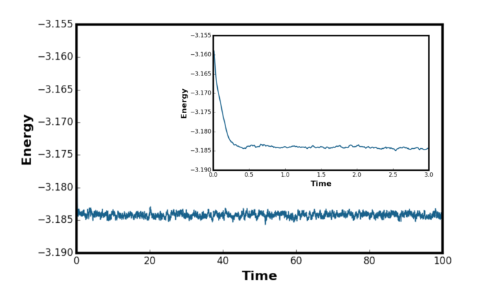
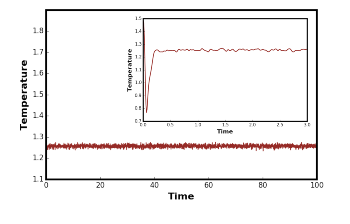
The system has reached equilibrium as the energy converges to a value. From Figures 4, 5 and 6 above, it is clear that the system reach equilibrium after 0.5 time in reduced units. The fluctuations were observed for energy, temperature and pressure but it was greatest for the pressure. The mean squared fluctuation in temperature is given by :

$⟨(\mathrm{\Delta }T{)}^2⟩=\frac{k_B{T}^2}{C_V}$

Therefore, the fluctuation is proportional to $C_V^{-\frac{1}{2}}$ and so decreases according to $1/\sqrt{N}$. Figure 7 shows the temperature plot for the equilibration where the system size was increased by a factor of ten. It can be clearly observed that the fluctuations in the system is much smaller as predicted by the relationship above.

Figure 8. Combined energy plot for system equilibrated using different timesteps 0.001, 0.0025, 0.0075, 0.01, 0.015

Figure 8 shows the energy plot for the system equilibrated using five different timesteps. Timestep of 0.015 would be particularly a bad choice as the total energy of the system fail to converge to a value. The divergence was due to the error occurring in the integration leading to unstable configurations as discussed in the previous section. For timesteps 0.0075 and 0.01, the system has converged to a wrong energy value. For the timesteps 0.001 and 0.0025, there was no observable difference in the converged energy value meaning that decreasing the timestep beyond 0.0025 is unlikely to have a significant effect on the simulation. In order to optimise the computational time, 0.0025 was the timestep chosen for the subsequent simulations. This is a very approximate approach to choosing the optimum timestep and literature search showed that there are mathematical proof available to what is the best timestep to use as shown by Choe et al. Tick

Running Simulations Under Specific Conditions

Task 1

The kinetic energy of the system without the correction is given by:

$E_K=\frac{3}{2}N{k}_{B}T=\frac{1}{2}\sum _i{m}_i{v}_i^2$

The kinetic energy of the system with the correction is given by:

${E_K}^{\prime }=\frac{1}{2}\sum _i{m}_i{v}_i^2{\gamma }^2$

${\gamma }^2\frac{1}{2}\sum _i{m}_i{v}_i^2=\frac{3}{2}N{k}_B\tau$

Sub $E_K$ into ${E_K}^{\prime }$

${\gamma }^2\frac{3}{2}N{k}_{B}T=\frac{3}{2}N{k}_B\tau$

$\gamma ={\left(\frac{\tau }{T}\right)}^{\frac{1}{2}}$ Tick

Task 2

Numbers 100, 1000 and 100000 corresponds to Nevery, Nrepeat and Nfreq from the LAMMPS manual and controls which timesteps will be used to calculate the average.. Nevery specifies the timestep interval, Nrepeat specify how may times to repeat the collection from the end, and Nfreq specifies how often the average will be printed. This setting would therefore take samples every 100 timestep for one thousand times and will generate one average at the end of the simulation as Nfreq = total timestep = 100000. Nevery * Nrepeat must always less or equal to Nfreq. Tick

Task 3

Figure 9. Density vs Temperature plot for MD simulation performed at 2.5 and 3.5 pressure in reduced units. Ideal gas plot is not shown.

Figure 10. Density vs Temperature plot for MD simulation performed at 2.5 and 3.5 pressure in reduced units. Ideal gas plot is also shown

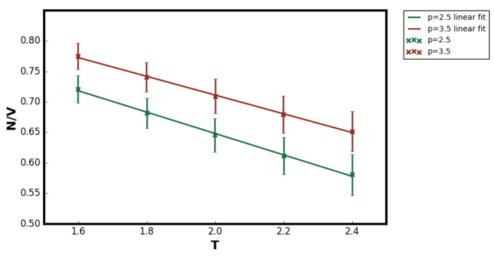
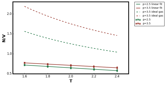
Figure 9 and Figure 10 shows the variation in density as for the temperature range 1.6 to 2.4. The error bar in x-direction was too small to be observed directly on the plot. In order to include the ideal gas relations in the plot, the equation must be converted to reduced units. Pressure has same units as energy over volume.

$$\begin{gathered} p=\frac{F \\ [kg \\ m \\ {s}^{-2}]}{A \\ [m^2]}=\frac{E \\ [kg \\ {m}^2 \\ {s}^{-2}]}{V \\ [m^3]}\frac{{\sigma }^3ϵ}{{\sigma }^3ϵ}=\frac{E^{*}ϵ}{V^{*}{\sigma }^3}=\frac{p^{*}ϵ}{{\sigma }^3} \end{gathered}$$

$D=\frac{D^{*}}{{\sigma }^3}$

$T=\frac{T^{*}ϵ}{k_B}$

Sub in the following relations into the ideal gas equation

$D=\frac{N}{V}=\frac{p}{k_{B}T}$

$\frac{D^{*}}{{\sigma }^3}=\frac{p^{*}ϵ}{{\sigma }^3}\frac{1}{k_B}\frac{k_B}{T^{*}ϵ}$

$D^{*}=\frac{p^{*}}{T^{*}}$

For the pair potential describing the interactions in simple liquids, the most important feature is the repulsions. Unlike gas, the interatomic separation in liquids are much smaller and hence the short-range repulsions characterises the liquid state. The attractive forces are long range and vary little with the distance forming a uniform background. The attractive interactions has a little role in determining the properties of the liquid state. Since the simulation was performed in the supercritical fluid region, it was expected that the repulsive interactions had more significant role than in the gaseous state. In the ideal gas model, there are no interactions between the particles and hence they would exist with smaller interatomic distances compared to the LJ supercritical fluid. This was the reasoning behind why the resulting density from LAMMPS simulation was lower than the ideal gas prediction for the entire temperature range tested.Tick

Figure 9 showed as the temperature increased, the density of the system decreased for both pressures at 2.5 and 3.5. This observation was due to the thermal expansion of the system; at higher temperatures the average kinetic energy of the system increasing as according to the equipartition equation derived in the previous section. Therefore the velocity of the particles increases which in turn increases the repulsive interactions between the atoms. Hence, the particles exists with greater interatomic separation compared to the lower temperature simulations and so the simulation box size increased in the NPT ensemble. It should also be noted that the agreement between the ideal gas and LAMMPS simulation results were better as the temperature increased. Due to this decrease in density at higher temperatures, the behaviour of the LAMMPS system was more ideal-gas like meaning the repulsive interaction had a less significant role. Similar reasoning would also explain why at lower pressure, the agreement between ideal gas and LAMMPS simulation was better (the difference between the dashed line and the solid line in Figure 10). At lower pressures, the interatomic separation increases and again the system became more ideal gas like.Tick

Extension 1

In this section, the pressure dependence of the system was investigated to justify the difference in repulsive and attractive interactions as presented in the previous section. The NPT equilibration was performed in the pressure range 0.1-1.5 reduced units and the corresponding density was calculated. Temperature remained constant at 2.0 for all simulations to ensure there were no phase transition. The LAMMPS simulation results were than compared to the ideal gas plot using the reduced ideal gas equation derived above.

Figure 11. Density of the system plotted as a function of pressure to compare LAMMPS simulation results with the reduced ideal gas equation

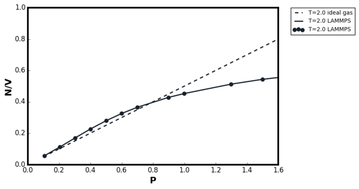
The result in Figure 11 can be divided into three regions; at very low pressures, the agreement between the ideal gas plot and the LAMMPS simulation results converged. In the pressure range 0.3-0.6, the LAMMPS simulation results showed greater density than it was predicted by the ideal gas equation, and finally at very high pressures, the LAMMPS simulation showed much lower density as according to TASK 3. At very low pressures, the system size was very large and hence most particles existed with the interatomic distances greater than the LJ cutoff specified in the LAMMPS simulation. Therefore, the interatomic interactions were minimal and the ideal gas was a good model to use. At the intermediate pressure range, the system size was small enough such that the interatomic forces became significant. However, since the attractive interaction has much longer range than the repulsive, the attractive forces dominated and hence, the LAMMPS simulation resulted in higher density than the ideal gas prediction. At higher pressures, the system size was sufficiently small for the repulsive interaction to take its effect and hence the density predicted by LAMMPS was lower than the ideal gas equation. Good

Calculating Heat Capacities Using Statistical Physics

The LAMMPS input script used to perform heat capacity measurements using NVE ensemble is shown below

### DEFINE SIMULATION BOX GEOMETRY ###
variable D equal 0.2

lattice sc ${D}
region box block 0 15 0 15 0 15
create_box 1 box
create_atoms 1 box

### DEFINE PHYSICAL PROPERTIES OF ATOMS ###
mass 1 1.0
pair_style lj/cut/opt 3.0
pair_coeff 1 1 1.0 1.0
neighbor 2.0 bin

### SPECIFY THE REQUIRED THERMODYNAMIC STATE ###
variable T equal 2.0
variable p equal 2.5
variable timestep equal 0.0025

### ASSIGN ATOMIC VELOCITIES ###
 velocity all create ${T} 12345 dist gaussian rot yes mom yes
    
 ### SPECIFY ENSEMBLE ###
 timestep ${timestep}
 fix nve all nve
    
 ### THERMODYNAMIC OUTPUT CONTROL ###
 thermo_style custom time etotal temp press
 thermo 10
    
 ### RECORD TRAJECTORY ###
 dump traj all custom 1000 output-1 id x y z
    
 ### SPECIFY TIMESTEP ###
    
 ### RUN SIMULATION TO MELT CRYSTAL ###
 run 10000
 unfix nve
 reset_timestep 0
    
 ### BRING SYSTEM TO REQUIRED STATE ###
 variable tdamp equal ${timestep}*100
 variable pdamp equal ${timestep}*1000
 fix nvt all nvt temp ${T} ${T} ${tdamp} # system simulated in nvt with a specific density
 run 10000
 unfix nvt
 fix nve all nve
 reset_timestep 0
    
 ### MEASURE SYSTEM STATE ###
 thermo_style custom step etotal temp press density atoms
 variable dens equal density
 variable dens2 equal density*density
 variable temp equal temp
 variable temp2 equal temp*temp
 variable press equal press
 variable press2 equal press*press
 variable energy equal etotal
 variable energy2 equal etotal*etotal
 variable no_atoms2 equal atoms*atoms
 fix aves all ave/time 50 2000 100000 v_dens v_temp v_press v_dens2 v_temp2 v_press2 v_energy v_energy2
 run 100000
    
 variable avedens equal f_aves[1]
 variable avetemp equal f_aves[2]
 variable avepress equal f_aves[3]
 variable errdens equal sqrt(f_aves[4]-f_aves[1]*f_aves[1])
 variable errtemp equal sqrt(f_aves[5]-f_aves[2]*f_aves[2])
 variable errpress equal sqrt(f_aves[6]-f_aves[3]*f_aves[3])
 variable heatcap equal ${no_atoms2}*((f_aves[8]-(f_aves[7]*f_aves[7]))/f_aves[5])
    
 print "Averages"
 print "--------"
 print "Density: ${avedens}"
 print "Stderr: ${errdens}"
 print "Temperature: ${avetemp}"
 print "Stderr: ${errtemp}"
 print "Pressure: ${avepress}"
 print "Stderr: ${errpress}"
 print "heatcap: ${heatcap}"

Figure 12. Variations in heat capacity at constant volume with increasing temperature for the LJ system simulated in LAMMPS. The simulation was performed for two different pressures 0.2 and 0.8

The observed heat capacities were to the order of $10^{-5}-10^{-4}$. Small heat capacity was expected as the measurements were performed in the NVE ensemble meaning the energy of the system was held constant and the fluctuations were very small. The heat capacity of the system decreased as the temperature increased for both pressure systems. The literature search showed that the reasoning behind this behaviour came from liquid potential-energy landscape with intervalley motion considerations. . The heat capacity at constant volume is given by:

$C_V={\left(\frac{\partial U}{\partial T}\right)}_V$

so in order to explain the behaviour, the change in the internal energy as a function of the temperature need to be considered. Consider the motion of one atom as a probe with all the other atoms fixed in space. To visualise the potential energy surface, the potential can be plotted vertically against the volume on the horizontal plane. Valleys and ridges will exist on the plane as the potential will be higher at the positions occupied by the atoms and the potential will be lower in open spaces (for liquids, the surface will not be regular compared to the solid). The mean potential for the probe ion can be considered as the average potential across the region which is reachable. At lower temperatures, there is insufficient energy in the system and hence the probe atom is restricted to the valleys. At higher temperatures, the probe can move freely over the entire potential energy surface. Therefore, the average potential for the probe will initially increase with the temperature but will eventually saturate at higher temperature range when the entire surface become reachable. Figure 13 illustrates this change in the mean potential per probe atom as a function of temperature. The literature showed that this limit corresponded to $\frac{1}{2}<\varphi >$ per atom.

Figure 13. The average potential per atom increases with temperature but saturates at higher temperature range when the entire potential energy surface is reachable

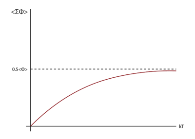
Since the heat capacity is given by the gradient of the potential, the reasoning above explains the decrease in heat capacity as the system cannot store additional thermal energy.

To explain the decrease in heat capacity the with density, the density of state (DOS) needs to be considered. DOS is given by

$DOS(E)=\left|\frac{dn}{dE}\right|$

where n is the number of states and E is the energy. DOS therefore reflects the number of states per given energy level interval. Since the number atoms per unit volume decreased with the decreasing density, the number of energy levels available per unit energy has also decreased. Hence, the increase in density has increased the DOS and the heat capacity increased as the system was able to store more energy. Tick

Extension 2

To properly investigate the change in the heat capacity as a function of temperature, the simulation should be carried out in NVT ensemble. To investigate the variation in heat capacity with temperature in NVT, 25 LAMMPS simulations were performed at 2.5 reduced unit pressure for the temperature range of 2.0-2.8.

Figure 14. The plot outlining the variations in heat capacity for the temperature range 2.0-2.8 for the NVT ensemble.

The results showed no noticeable trend and the heat capacity fluctuated for the entire temperature range. The possible cause could be due to the small system size, and therefore the number of samples were not representative of the population. However, due to the long simulation time for larger systems, no further NVT investigation was performed. Good

Radial Distribution Function

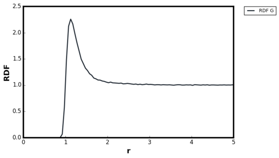
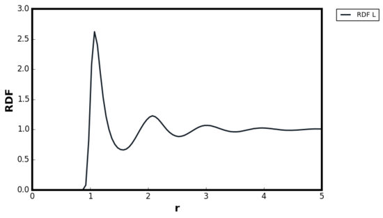
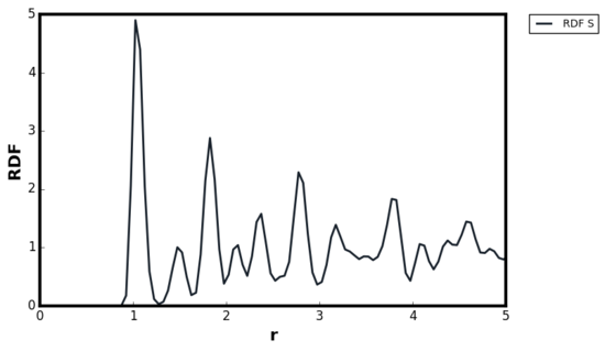
The radial distribution function for the LJ system was calculated for solid, liquid and gaseous states using the phase diagram determined by Lin et al.

Figure 15. Radial distribution function for the gaseous system calculated at D=0.02, T=1.20			Figure 16. Radial distribution function for liquid system calculated at D=0.80, T=1.20
Figure 17. Radial distribution function for the solid system calculated at D=1.20, T=0.10			Figure 18. Radial distribution function for the solid system calculated at D=1.20, T=1.00

The correlation function g(r), is defined as:

$g(r)=\frac{\rho (r)}{{\rho }^{\prime }}$

where $\rho$ and ${\rho }^{\prime }$ respectively corresponds to the local density at distance r and the bulk average density. Since the bulk density is the statistical average of the system, g(r) can represent the degree of order between the central particle and the surrounding species at distance r. If all species and the central particle at the origin are independent at r, simply $\rho ={\rho }^{\prime }$ and hence g(r) would equal 1. ,

Figure 19. The combined RDF form Figure 15, 16 and 17

Figure 20. The running integral for RDF calculated for solid, liquid and gaseous systems

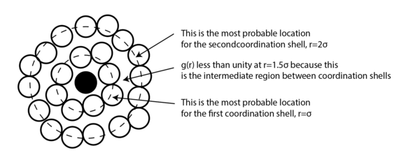
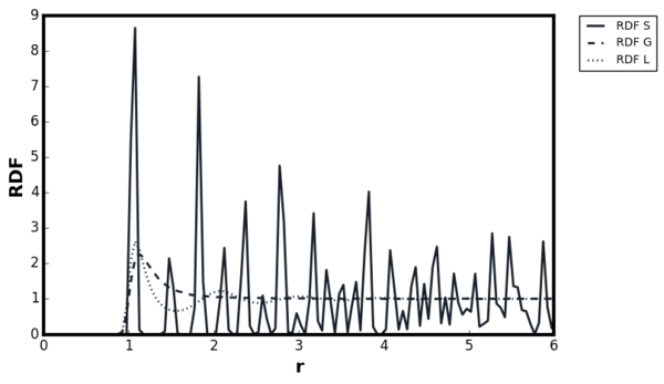
For all three systems, $g(r)=0$ when $r<\sigma$. $\sigma$corresponded to the separation at which the LJ potential became positive and hence, no atoms can exist at the distance less than this value. For the dense fluid, the first coordination shell, or the nearest neighbour, existed at $r=\sigma$ and since reduced units were used, the first peak indeed occurred at 1. The second peak was observed again at $r=2\sigma$ which corresponded to the second coordination shell. The distance $r=1.5\sigma$, corresponded to the intermediate region between the first and second coordination shell and hence g(r) was less than unity. The oscillatory behaviour was observed since some long range order was present in liquids. At very long distances, the g(r) converged to 1, meaning there was no order present between the central atom and the species at r. Tick

For the gaseous system, one peak was observed around $r=\sigma$ but g(r) quickly converged to 1 beyond $r=2\sigma$. As proven in the previous section, when the density of the system is low, the attractive interactions are more significant than repulsions and hence the local density was initially higher than the bulk. The range of correlation corresponded to the cutoff distance of $3\sigma$ as stated in the input file and therefore, no oscillatory behaviour was observed due to the short range order in the system. The behaviour of the liquid and gaseous systems agreed well with the MD study performed by Morsali et al.

Figure 21. The digram of a liquid system outlining the reasoning behind the peaks observed in the liquid RDF plot

Figure 22. The diagram of a solid system outlining the reasoning behind the peaks observed in the solid RDF plot

For ideal solids, a delta function was expected at the lattice points corresponding to the location of the atoms, and g(r) = 0 in interatomic locations. The behaviour was in contrast with liquid where g(r) ≠ 0 at $r=1.5\sigma$, indicating the difficulty of diffusion in solids. However, some degree of broadening was always present above 0K due to the thermal vibrations. The Figures 17 and 18 illustrated this broadening effect as g(r) for Figure 18 was calculated at higher temperature than Figure 17. The Monte Carlo study by Choi et al, showed first three peaks located at 1.0125, 1.4575 and 1.7625, therefore the simulation results agreed with the literature. Tick

The coordination number is given by the following relationship

$N(r)=4\pi \rho \underset{0}{\overset{r}{\int }}{r}^{2}g(r)dr$

Therefore, the number integral of the first peak in Figure 20 represents the coordination number, corresponding to the first plateau in Figure 21. The number of atoms in the first coordination shell was found to be 12. Since all atoms in FCC lattice are equivalent, the coordination number for each first three peaks were also 12, as expected for maximum packing efficiency of FCC lattice. It is important to note that the number of atoms in the first coordination shell corresponds to the area under the peak not the height. Indeed, the number of atoms in the first coordination shell also corresponded to 12 (running integral read at r = 1.5). The difference in the number integral between the current peak integral value and the previous peak integral represents the number of atoms in each coordination shell. The maximum packing efficiency for the liquid and the solid systems ensured that the repulsions were minimised and also supported the argument that the atoms behave like 'hard-core' in LJ potential model.Tick

Table 1. A summary of the RDF results from LAMMPS simulations for liquid, gas and solid LJ systems

	peak 1	peak 2	peak 3
vector	$d$	$r_1$	$r_2$
Miller indices	[0, 1/2, 1/2]	[1,0,0]	[1, 1/2, 1/2]
relative magnitude to d	$1\sigma$	$\sqrt{2}\sigma$	$\sqrt{3}\sigma$
Running Integral	12	18	42
Number of atoms in each shell	12	6	24
Coordination number	12	12	12

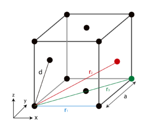
The lattice spacing corresponds to the nearest neighbour distance which was given by vector d:

$d=\sqrt{{\left(\frac{a}{2}\right)}^2+{\left(\frac{a}{2}\right)}^2}=\frac{a}{\sqrt{2}}$

Hence the relative magnitudes of other vectors can be calculated as:

$\frac{r_1}{d}=a\times \frac{\sqrt{2}}{a}=\sqrt{2}$

$r_2=\sqrt{a^2+{\left(\frac{a}{2}\right)}^2+{\left(\frac{a}{2}\right)}^2}=\frac{a\sqrt{3}}{\sqrt{2}}$

$\frac{r_2}{d}=\frac{a\sqrt{3}}{\sqrt{2}}\times \frac{\sqrt{2}}{a}=\sqrt{3}$Tick

The position of the first three peaks in solids were much closer to the central atom compared to liquid and gases. This decrease from $2\sigma$ distance in liquids was due to the bulk density of solid being higher than liquids. . Furthermore, for solids g(r) did not converged to 1 within the range of r where the experiment was performed. The reasoning came from the fact that the first coordination shell was more ordered in solids than liquids. Ordering prohibited any species existing between the first two coordination shell and gave rise to the long range order in the subsequent coordination shells.Good

Figure 23. The OVITO simulation of liquid, solid and gaseous LJ systems

Diffusion

Task 1

Figure 24. Mean squared distribution plots for solid and liquid LJ systems			Figure 25. Mean squred distribution plots for solid, liquid and gaseous LJ systems simulated with 1 million atoms
Figure 26. Mean squared distribution plot for gaseous LJ systems with different densities			Figure 27. Calculated diffusion coefficients for different density gaseous systems

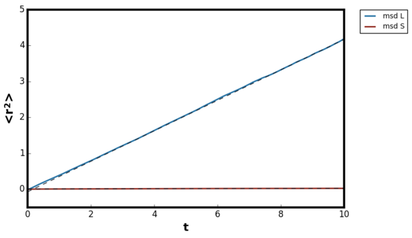
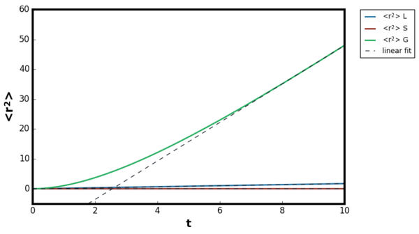
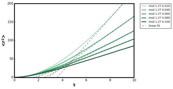
The mean squared displacement plot showed the expected trend, for the inertial regime the increase was non-linear but at the diffusive regime the relationship became linear for liquid, gas and solids. For the gaseous plot, longer timestep was required compared to solids and liquids before the trend became linear. The diffusion coefficient was calculated by fitting a linear line of best fit in the linear region. For the gaseous systems, the calculated diffusion coefficient varied depending on the density the simulation was ran. Therefore, five simulations were performed at the density range 0.02-0.10 at constant T=1.2 and the calculated diffusion coefficients are shown in Figure 27.Tick

The inertial regime arises because when the particle initially start to move, their trajectories are unaltered as they do not encounter any neighbours. The motion of the atoms are much complex in this region but can be qualitatively simplified as the following. Since the collision is minimal, the velocity of the atoms remain almost constant. Hence, the distance the particles travel is approximately proportional to the time, and therefore the mean squared displacement is quadratic. In the diffusive regime, the motion of the particle resemble the random walk due to the fluctuating forces from the environment. Therefore, in diffusive motion the particle progress much less displacement per unit time than the inertial motion and obeys the Einstein equation.

Calculated diffusion coefficients were compared to the study by Rowley et al. and are summarised below. The dimensionless diffusion coefficient was given by:

$D^{*}=D\sqrt{\frac{ϵ}{m{\sigma }^2}}$

Table 2. A summary of the diffusion coefficient calculated for LJ system with literature values from Rowley et al. All units are in ${r^{*}}^2/timestep$

	${\rho }^{*}=1.20,T=1.0$ [Solid]	${\rho }^{*}=0.80,T=1.0$ [Liquid]	${\rho }^{*}=0.10,T=1.2$ [Gas]
This Study	$2.683\times 10^{-4}$	$0.071$	$1.694$
Rowley et al.		$0.065$	$1.681$Tick

The results from this simulation lied within 10% from the literature value. Both results showed that for the solids the diffusion coefficient was close to zero, and a higher value for gas compared to liquid. The average velocity of particles in gaseous system is higher than liquid and therefore the atoms are able to travel further in the given timestep leading to higher diffusion coefficient. Rowley et al used different system size, LJ cutoff value and different simulation time which were the main cause of the discrepancy.

The diffusion coefficient calculated from 1 million system size corresponded to $1.074$, $0.030$ and $3.035\times 10^{-6}$ for gaseous, liquid and solid systems respectively. Direct comparison with the previous simulation result was not possible as the output file did not state density and temperature the readings were taken. As shown in Figure 27, even within the same phase, the diffusion coefficient changes with different density and temperature.Tick

Task 2

The position and the velocity of the harmonic oscillator is given by:

$X(t)=Acos(\omega t+\varphi )$

$V(t)=-A\omega sin(\omega t+\varphi )$

Velocity autocorrelation function is given by:

$C(\tau )=\frac{\underset{-\mathrm{\infty }}{\overset{\mathrm{\infty }}{\int }}V(t)V(t+\tau )dt}{\underset{-\mathrm{\infty }}{\overset{\mathrm{\infty }}{\int }}{V}^2(t)dt}$

$C(\tau )=\frac{(A\omega {)}^2\underset{-\mathrm{\infty }}{\overset{\mathrm{\infty }}{\int }}sin(\omega t+\varphi )sin(\omega t+\omega \tau +\varphi )dt}{(A\omega {)}^2\underset{-\mathrm{\infty }}{\overset{\mathrm{\infty }}{\int }}si{n}^2(\omega t+\varphi )dt}$

use identity

$sin(\omega t+\omega \tau +\varphi )=sin(\omega t+\varphi )cos(\omega t)+cos(\omega t+\varphi )sin(\omega \tau )$

$C(\tau )=\frac{cos(\omega \tau )\underset{-\mathrm{\infty }}{\overset{\mathrm{\infty }}{\int }}si{n}^2(\omega t+\varphi )dt}{\underset{-\mathrm{\infty }}{\overset{\mathrm{\infty }}{\int }}si{n}^2(\omega t+\varphi )dt}+\frac{sin(\omega \tau )\underset{-\mathrm{\infty }}{\overset{\mathrm{\infty }}{\int }}sin(\omega t+\varphi )cos(\omega t+\varphi )dt}{\underset{-\mathrm{\infty }}{\overset{\mathrm{\infty }}{\int }}si{n}^2(\omega t+\varphi )dt}$

let

$I_1=\frac{cos(\omega \tau )\underset{-\mathrm{\infty }}{\overset{\mathrm{\infty }}{\int }}si{n}^2(\omega t+\varphi )dt}{\underset{-\mathrm{\infty }}{\overset{\mathrm{\infty }}{\int }}si{n}^2(\omega t+\varphi )dt}$

$I_2=\frac{sin(\omega \tau )\underset{-\mathrm{\infty }}{\overset{\mathrm{\infty }}{\int }}sin(\omega t+\varphi )cos(\omega t+\varphi )dt}{\underset{-\mathrm{\infty }}{\overset{\mathrm{\infty }}{\int }}si{n}^2(\omega t+\varphi )dt}$

use identity:

$si{n}^2(\theta )=\frac{1}{2}-\frac{1}{2}cos(2\theta )$

$I_1=\frac{cos(\omega \tau )\underset{-\mathrm{\infty }}{\overset{\mathrm{\infty }}{\int }}\frac{1}{2}-\frac{1}{2}cos(2\omega t+2\varphi )dt}{\underset{-\mathrm{\infty }}{\overset{\mathrm{\infty }}{\int }}\frac{1}{2}-\frac{1}{2}cos(2\omega t+2\varphi )dt}$

$I_1=\frac{cos(\omega \tau ){[\frac{1}{2}t-\frac{1}{4\omega }sin(2\omega t+2\varphi )]}_{-\mathrm{\infty }}^{\mathrm{\infty }}}{{[\frac{1}{2}t-\frac{1}{4\omega }sin(2\omega t+2\varphi )]}_{-\mathrm{\infty }}^{\mathrm{\infty }}}$

compared to t term, the sine term will be negligible in the limit of the integral

$I_1=\frac{cos(\omega \tau ){\left[\frac{1}{2}t\right]}_{-\mathrm{\infty }}^{\mathrm{\infty }}}{{\left[\frac{1}{2}t\right]}_{-\mathrm{\infty }}^{\mathrm{\infty }}}$

the divergence is the same on the denominator and the nominator and hence it is possible to cancel the integral

$I_1=cos(\omega \tau )$

now consider the second integral. Use identity:

$sin(2\theta )=2sin(\theta )cos(\theta )$

$I_2=\frac{sin(\omega \tau )\underset{-\mathrm{\infty }}{\overset{\mathrm{\infty }}{\int }}sin(2\omega t+2\varphi )dt}{\underset{-\mathrm{\infty }}{\overset{\mathrm{\infty }}{\int }}si{n}^2(\omega t+\varphi )dt}$

$sin(2\omega t+2\varphi )$ has $C_2$ rotational symmetry about the z axis and therefore the area over the x-axis is same as the area under the x-axis. Therefore, since the top and bottom limits are the same and the function also possesses the rotational symmetry, the positive area must equal negative area and hence the integral evaluates to zero.

$\underset{-\mathrm{\infty }}{\overset{\mathrm{\infty }}{\int }}sin(2\omega t+2\varphi )dt=0$

therefore

$I_2=0$

overall

$C(\tau )=cos(\omega t)$ Tick

Figure 28. A plot of sine function to illustrate the rotational symmetry of the system about the z axis

Task 3

Figure 29. A plot of VACF against timestep for the harmonic oscillator, LJ liquid and LJ solid systems

Figure 30. A plot of VACF against timestep for the LJ gaseous systems

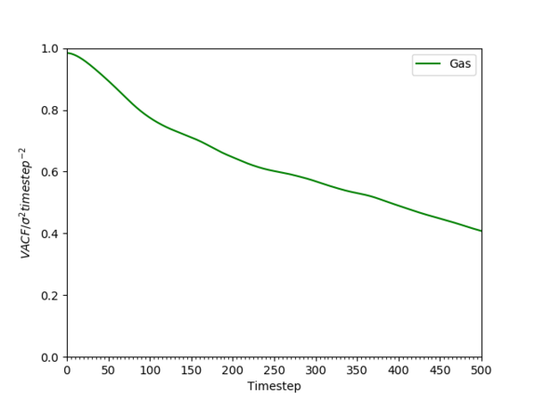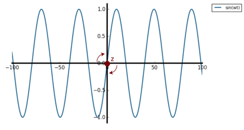
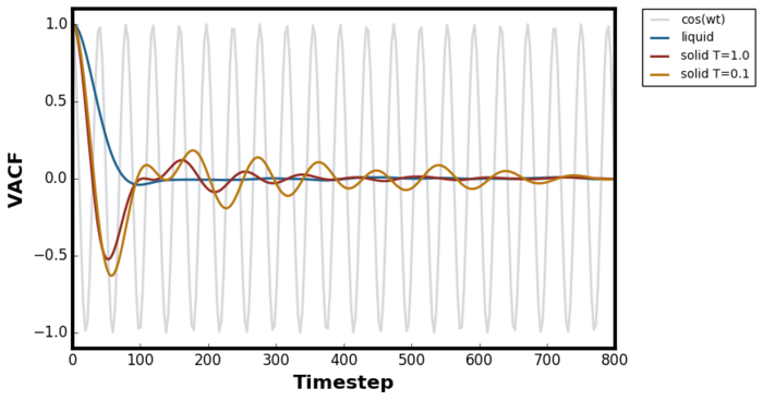
Figure 29 shows the normalised VACF for liquid and solids at two different temperatures compared to the VACF of the harmonic oscillator derived in the previous task. The Green-Kubo formalism is a popular method of choice for diffusion coefficient calculation and is given as:

$D=\frac{1}{3}\underset{t\to \mathrm{\infty }}{\lim }\underset{0}{\overset{T}{\int }}C(\tau )dt$

$C(\tau )=⟨\frac{1}{N}\sum _{i=1}^N{v}_i(0)\cdot v_i(t)⟩$

where the angle brackets indicate averaging over the statistical ensemble.

$C(\tau )$ is a measure of how well the velocity at time 0 correlate to velocity at time t. If there was a perfect correlation between velocity at t=0 and t, the product inside the angled bracket would always yield the same value and hence $⟨v_i(0)\cdot v_i(t)⟩$ →$⟨v_i^2(0)⟩$ and normalisation would result 1. If there is a no correlation $⟨v_i(0)\cdot v_i(t)⟩$ → $0$ since the product inside the bracket will result in random values and hence the average over the ensemble is zero. For large t, the correlation function will tend to zero if the property of the system is statistically averaged out by the internal motions.

For the simple harmonic oscillator, the VACF is simply a cosine wave and the correlation is always one after each oscillation cycle because the particle always return to the original position with the same initial velocity. Therefore the velocity is perfectly correlated at every one period, perfect negative correlation at every half period and no correlation at a quarter and three quarter of the period. The harmonic motion can be represented as a projection of a circular motion on one axis and is schematically represented in Figure 31 below.Tick

Figure 31. A diagram illustrating the reasoning behind the observed VACF for the harmonic oscillator

Solid, liquid and gaseous systems showed very different VACFs for the reasonings outlined below. It is important to differentiate two different type of motions in the system; oscillatory and diffusive, and the dominance of one of the two motions will ultimately determine the shape of VACF. Oscillatory motion dominance will result in VACF resembling the harmonic oscillator as the atoms go back to the original position whereas diffusion dominance will result in VACF exponentially decaying as the system is statistically averaged out quickly.

For gaseous systems, VACF simply decayed exponentially as the Brownian motion dominated and due to the large interatomic distances, oscillatory behaviour was not possible. This system took the longest for VACF to reach zero because due to the small density the number of hard collision per unit time was less than the solid or liquid. For liquid systems, a characteristic minima was observed followed by the negative correlation region before decaying to zero. The literature search showed that this was a well known phenomenon known as the "cage effect". The rebounding collision initially dominate over the scattering collision due to the high density of the liquid compared to the gaseous system. Therefore, the surrounding medium initially force oscillation over diffusion and each atom became locked in this "cage". However, frequent hard-core collisions in LJ liquid leads to quick statistical averaging and asymptotic decay of VACF to zero. For this system, the minima represented the timestep at which all particles have underwent at least one collision.Tick

In solids, the oscillatory behaviour dominates for longer duration as all the atoms are locked at the lattice site meaning there were no room for diffusion. For this system, the minima represented the timestep at which all particles have underwent at least one oscillation. Due to much higher packing efficiency in solid, the atoms are closer to each other than the liquid system and hence the observed minima occurred at earlier timestep. Furthermore, at lower temperature the minima was lower than the higher temperature VACF. This was due to the fact that the motion of the atoms were slower at lower temperature meaning it took longer time for statistical averaging to dominate. The fact that the period of the oscillation for solid at lower temperature was longer also supported this argument of slower motion.Tick

Figure 32. Running integral for the liquid and solid LJ systems for this study			Figure 33. Running integral for the gaseous LJ system for this study
Figure 34. Running integral for the liquid and solid LJ systems simulated with 1 million atoms			Figure 35. Running integral for the gaseous LJ system simulated with 1 million atoms

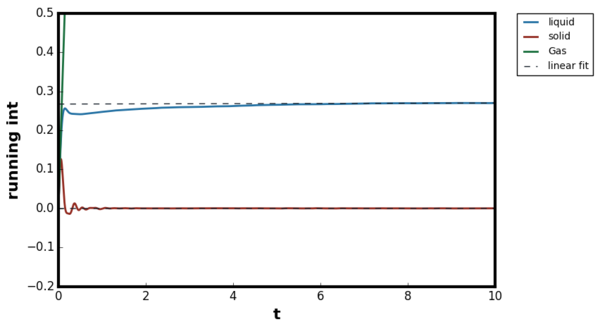
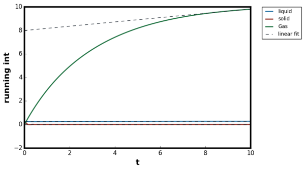
The diffusion coefficients were found by performing a linear fit at the plateaued region and extrapolating back to the y-intercept. For 1 million atom system size, it was not possible to perform the linear fit for the gaseous system as the system did not reach the diffusion regime within the timestep the experiment was performed. The results from Green-Kubo methods are summarised below

Table 3. A summary of the diffusion coefficient calculated for LJ system using the Green-Kubo methods. All units are in ${r^{*}}^2/timestep$

	[Solid]	[Liquid]	[Gas]
This study	$1.186\times 10^{-4}$	$0.081$	$1.645$
1 million atoms system size	$1.006\times 10^{-4}$	$0.009$

Comparing these results to the literature value from Task 1, Green-Kubo (G-K) method computed the diffusion coefficient of the liquid less accurately than the mean-squared displacement method. Literature search showed that G-K method was well known for overestimating the transport coefficient. . There are both advantages and disadvantages for both methods. The main disadvantage of the G-K method was that, a very large system size was required. The comparison of Figures 32 and 34 revealed that for the larger system, the oscillations were smaller and the plateauing region was much more clearly defined. Furthermore, periodic boundary conditions altered the coordinates of the atom back to the original simulation box whereas in reality, the atom would move to the next box and therefore affect the velocity correlation calculations. These two factors would mean a longer computational time was required for the G-K method.Tick

Extension 3

Motivation

Study by Hansen et al claimed to have observed the van der Waal's loop for the LJ model. It was therefore an interest to compare the current simulation results with this study to investigate the pressure dependence of the system as a function of density. This dependence was then compared with the van der Waal's equation to explore the validity of the equation to model the LJ system.

Methodology

The van der Waal's equation was modified to reduced units as follows:

$p=\frac{NkT}{V-Nb}-\frac{a{N}^2}{V^2}$

$p=\frac{p^{*}ϵ}{{\sigma }^3}$

$T=\frac{T^{*}ϵ}{k}$

$V=V^{*}{\sigma }^3$

$a=\frac{2\pi r^3}{3}{u}_0$

$r_{eq}=\sigma 2^{\frac{1}{6}}$

$E=E^{*}ϵ$

therefore

$a=\frac{2\sqrt{2}\pi r_{eq}^3}{3}{u}_0^{*}{\sigma }^3ϵ$

$a=a^{*}\sigma ϵ$

now sub in everything to van der Waal's equation

$\frac{p^{*}ϵ}{{\sigma }^3}=\frac{Nk{T}^{*}ϵ}{k}\frac{1}{V{\sigma }^3}-\frac{a{N}^2{\sigma }^3ϵ}{V^2{\sigma }^6}$

$p^{*}=\frac{N{T}^{*}}{V^{*}}-\frac{a^{*}{N}^2}{(V^{*}{)}^2}$

$p^{*}={\rho }^{*}T*-({\rho }^{*}{)}^2{a}^{*}$

The b term was set to zero as in LAMMPS simulations all atoms were treated as point particles. The values of a and N were kept identical to the parameters used in the LAMMPS simulations.

Results and Discussion

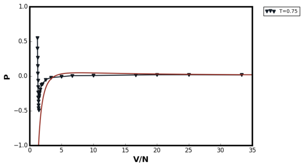
The results of the simulation are summarised in Figures 36 and 37 below:

Figure 36. A plot of LAMMPS simulation and van der Waal's equation at low temperature

Figure 37. A plot of LAMMPS simulation and van der Waal's equation at low temperature

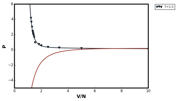The two figures above showed that van der Waal's equation agreed well for both temperatures at low densities as the system approached ideality. At T=1.5, no van der Waal's loop was observed. At T=0.75 the loop was observed due to the phase transition. At the first glance, the behaviour of the van der Waals equation at high density does not make sense. The equation predicted that the pressure would decrease as the volume of the system decrease. This was due to the fact that modelling the system as point particle was an extremely poor approximation to make in the van der Waal's equation at high density. The plot below shows the van der Waal's plot for constant temperature, number of particles, and the constant a but with varying b term.

Figure 36. van der Waal's isotherm for different values of b term

Comparing the van der Waal's equation with Figure 36, it can be seen that as the value of the b term decreased, the vertical asymptote was moved in the negative x direction and therefore the $V^2$ term began to dominate at low densities. This domination forced the pressure to become more negative as the volume decreased. Therefore, modelling the LAMMPS simulation with van der Waal's equation where all atoms were point particles was a not a good idea at high densities.

The isothermal compressibility is given by the following equation:

$\beta =-\frac{1}{V}{\left(\frac{\partial V}{\partial p}\right)}_T$

The Figure below compared the plot of dp/dV against density between the van der Waal's equation and the LAMMPS simulation result. The derivative of the pressure and volume was calculated by fitting a curve to the results in Figure 37.

Figure 37 Isothermal compressiblity predicted by van der Waal's equation and LAMMPS simulation

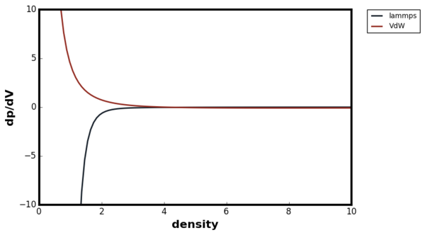
Again, the van der Waal's equation agreed very well with the LAMMPS simulation results at low densities. However, at high densities the van der Waal's equation predicted a completely unintuitive result; the system became more easier to compress at high densities. Again, this was due to the fact that b term was set to zero in the equation. Therefore, the van der Waal's equation was not a good model to use for point particle system at high densities.Good