JC: General comments: All tasks attempted with a few mistakes. Try to make your written explanations clearer and more focused to show that you understand what your results show and why.

Liquid Simulations^[1]

Introduction to Molecular Dynamics

The Classical Particle Approximation

TASK: Open the file HO.xls. In it, the velocity-Verlet algorithm is used to model the behaviour of a classical harmonic oscillator. Complete the three columns "ANALYTICAL", "ERROR", and "ENERGY": "ANALYTICAL" should contain the value of the classical solution for the position at time $t$ , "ERROR" should contain the absolute difference between "ANALYTICAL" and the velocity-Verlet solution (i.e. ERROR should always be positive -- make sure you leave the half step rows blank!), and "ENERGY" should contain the total energy of the oscillator for the velocity-Verlet solution. Remember that the position of a classical harmonic oscillator is given by $x (t) = A \cos (ω t + ϕ)$ (the values of $A$ , $ω$ , and $ϕ$ are worked out for you in the sheet).

By referring to Fig.1 (below), the analytical solution to the harmonic oscillator has been calculated using the formula using the formula $x (t) = A \cos (ω t + ϕ)$ above using the data provided. As shown, the error was calculated by taking the absolute value of the results from the analytical and Velocity-Verlet solutions. Lastly, the total energy was also calculated by adding together the potential and kinetic energies of the harmonic oscillators. The kinetic energy of the oscillator can be given by $E_{k} = \frac{1}{2} m v^{2}$ where $E_{k}$ is the total kinetic energy of the system, $m$ is the mass of the oscillator and is treated as constant throughout the simulation. $v$ is the velocity at which the particle is vibrating at that moment in time. The potential energy of the system may be given by integrating Hooke's Law (allowed since the system is being treated classically), $F = - k L$ from $0$ to $L$ with respect to $L$ , yielding $V = \frac{1}{2} k L^{2}$ ; where $V$ is the potential energy, $k$ is the force constant and $L$ is the displacement of the atoms from their equilibrium positions. Hence the total energy of the system may be given as:

E_{T O T A L} = E_{k} + V = \frac{1}{2} m v^{2} + \frac{1}{2} k L^{2}

(1)

TASK: For the default timestep value, 0.1, estimate the positions of the maxima in the ERROR column as a function of time. Make a plot showing these values as a function of time, and fit an appropriate function to the data.

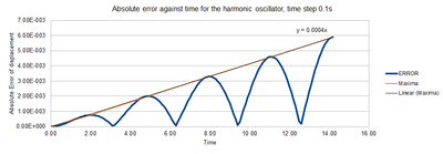
The positions of the maxima can be found by looking at the Error-Time graph, and then extracting a the highest value from near this time period. These plots can then form a linear fit across the maxima curve (Table 1 and Fig. 2)

Table 1
Time	Error
0.00	0.000000
2.00	0.000758
4.90	0.002008
8.00	0.003301
11.10	0.004604
14.20	0.005911

The graph clearly shows that there is a linear increase in the error with time by a factor of 0.004. This shows that as time increases, the error increases as there is a greater difference between the displacement in the analytical and approximate solutions. Consequently, the analytical and velocity-Verlet algorithm only deliver results with low errors when time is close to 0.

JC: Why does the error oscillate?

TASK: Experiment with different values of the timestep. What sort of a timestep do you need to use to ensure that the total energy does not change by more than 1% over the course of your "simulation"? Why do you think it is important to monitor the total energy of a physical system when modelling its behaviour numerically?

At $t = 0$ , the total energy of the system is 0.500 (this is a maximum). A 1% deviation from this value would mean that there tolerance of 0.005; i.e. the energy may lie anywhere between 0.495 and 0.500 to satisfy the query. At large timesteps (e.g 0.500, there is a deviation greater than 1%, however as we decrease this incrementally by 0.1, a timestep of 0.200 delivers the energies within a tolerance of 1%.

It is important to monitor the total energy of the system is to ensure that the the 1st law of thermodynamics is obeyed (i.e. the total energy of the system is the same before and after applying work). When using numerical techniques, several approximations are applied and so this law may sometimes be broken. It is therefore critical to monitor the total energy to prevent this from occurring.

JC: God choice of timestep.

Atomic Forces

TASK: For a single Lennard-Jones interaction, $ϕ (r) = 4 ϵ (\frac{σ^{12}}{r^{12}} - \frac{σ^{6}}{r^{6}})$ , find the separation, $r_{0}$ , at which the potential energy is zero. What is the force at this separation? Find the equilibrium separation, $r_{e q}$ , and work out the well depth ( $ϕ (r_{e q})$ ). Evaluate the integrals $\int_{2 σ}^{\infty} ϕ (r) d r$ , $\int_{2.5 σ}^{\infty} ϕ (r) d r$ , and $\int_{3 σ}^{\infty} ϕ (r) d r$ when $σ = ϵ = 1.0$ .

1) When the potential energy is zero,

ϕ (r) = 0

; it follows that:

0 = 4 ϵ [\frac{σ^{12}}{r_{o}^{12}} - \frac{σ^{6}}{r_{o}^{6}}]

By diving through by

4 ϵ

and then rearranging, it can be seen that:

\frac{σ^{12}}{r_{o}^{12}} = \frac{σ^{6}}{r_{o}^{6}}

By cancellation and rearranging, the following result is obtained when the potential is zero:

σ = r_{o}

(2)

2) In order to find the force when Eqn. 2 above holds true, the Lennard-Jones Potential,

ϕ (r)

, is differentiated with respect to

r

:

F = \frac{d ϕ (r)}{d r} = 4 ϵ [\frac{6 σ^{6}}{r^{7}} - \frac{12 σ^{12}}{r^{13}}]

Now insert the result from Eqn. 2 into the above and cancel down:

F = 4 ϵ [\frac{- 6}{σ}] \Rightarrow F = \frac{- 24 ϵ}{σ}

(3)

3) To find the equilibrium separation,

r_{e q}

,

ϕ (r)

must be differentiated with respect to

r

but recall that at equilibrium separation, the force is equal to 0:

F = \frac{d ϕ (r)}{d r} = 4 ϵ [\frac{6 σ^{6}}{r^{7}} - \frac{12 σ^{12}}{r^{13}}] = 0

But after dividing by

4 ϵ

and rearranging, it can clearly be seen that:

\frac{12 σ^{12}}{r^{13}} = \frac{6 σ^{6}}{r^{7}}

which after rearranging yields the result

r_{e q} = 2^{\frac{1}{6}} σ

(4)

4) The first integral may be evaluated as follows:

4 ϵ \int_{2 σ}^{\infty} [\frac{σ^{12}}{r_{o}^{12}} - \frac{σ^{6}}{r_{o}^{6}}] d r = 4 ϵ σ^{12} [\frac{r^{- 11}}{- 11}]_{2 σ}^{\infty} - 4 ϵ σ^{6} [\frac{r^{- 5}}{- 5}]_{2 σ}^{\infty}

After substitution of

ϵ = σ = 1.0

, and

\infty = a

, it follows after calculation that:

\frac{1}{5632} - \frac{1}{40} + \lim_{a \to \infty} [\frac{4}{5 a^{5}} - \frac{4}{11 a^{11}}]

As

a

tends to infinity, the fractions within the limit tend to 0. As a result:

\int_{2 σ}^{\infty} ϕ (r) d r = - 2.48 \times 1 0^{- 2} (3 s f)

By the same method, the other two integrals may be evaluated as:

\int_{2.5 σ}^{\infty} ϕ (r) d r = - 8.18 \times 1 0^{- 3} (3 s f)

and

\int_{3 σ}^{\infty} ϕ (r) d r = - 3.29 \times 1 0^{- 3} (3 s f)

From the results, as the value of the lower integral limit increases, the area enclosed by the Lennard Jones curve decreases. This makes sense, since as the distance between two atoms increases, the potential energy decreases.

JC: All maths correct and nicely laid out, what about the well depth ( $ϕ (r_{e q})$ )?

Periodic Boundary Conditions

TASK: Estimate the number of water molecules in 1ml of water under standard conditions. Estimate the volume of $10000$ water molecules under standard conditions.

The concentration of pure water is 55.5 moldm^-3. The number of moles is equal to: $m o l e s = 55.5 \times \frac{1}{1000}$ . Which we then multiply by Avogadro's number to find $3.34 \times 1 0^{22}$ water molecules in 1mL of water. To find the volume of 10,000 water molecules, the same principles can be applied as above to find that $2.99 \times 1 0^{- 19} m L$ is the volume which they would occupy.

TASK: Consider an atom at position $(0.5, 0.5, 0.5)$ in a cubic simulation box which runs from $(0, 0, 0)$ to $(1, 1, 1)$ . In a single timestep, it moves along the vector $(0.7, 0.6, 0.2)$ . At what point does it end up, after the periodic boundary conditions have been applied?.

To solve this problem, simply add the two vectors together: $(0.5, 0.5, 0.5) + (0.7, 0.6, 0.2) = (1.2, 1.1, 0.7)$ However, the boundary of the box is $(1, 1, 1)$ so the molecule will appear on the other side of the box if any of the x,y or z components are greater than 1. Therefore it follows that the molecule's final position is $(0.2, 0.1, 0.7)$

JC: Correct.

Reduced Units

TASK: The Lennard-Jones parameters for argon are $σ = 0.34 n m, ϵ / k_{B} = 120 K$ . If the LJ cutoff is $r^{*} = 3.2$ , what is it in real units? What is the well depth in ${k J m o l}^{- 1}$ ? What is the reduced temperature $T^{*} = 1.5$ in real units?

From the wiki task page, it is given that $r^{*} = \frac{r}{σ}$ . Hence, by substitution of $σ = 0.34 n m$ and $r^{*} = 3.2$ , the value of $r$ can be calculated to yield $1.09 n m (3 s f)$ as the answer.

Substitution of the result above for the value of $r$ and $σ$ into the Lennard Jones potential gives the following: $ϕ (r) = - 3.25 \times 1 0^{- 14} J$ . However to find the well depth in $k J m o l^{- 1}$ , the answer is divided by 1000 and multiplied by Avogadro's number. The final answer is therefore $- 1.97 \times 1 0^{7} k J m o l^{- 1} (3 s f)$ .

Again, by using the equation given; $T^{*} = \frac{k_{b} T}{ϵ}$ and the data provided, the real temperature can be calculated as $0.0125 K$

JC: Value of r is correct, but the well depth and temperature are not. The well depth is just epsilon, so you just need to convert the value of epsilon that you're given, epsilon = 120K*kB, into kJmol-1. The temperature is 1.5*120 = 180K.

Equilibration

Output of the first simulation

Creating the Simulation box

TASK: Why do you think giving atoms random starting coordinates causes problems in simulations? Hint: what happens if two atoms happen to be generated close together?

If two atoms are generated close together, then they will both have a very high potential energy. The worst case scenario is if the system generates the atoms very close together - so much so that they are almost superposed. This this case, the Lennard-Jones potential energy would tend to infinity, which would cause problems when running the simulation.

JC: The high repulsion between atoms will cause the simulation to crash.

TASK: Satisfy yourself that this lattice spacing corresponds to a number density of lattice points of $0.8$ . Consider instead a face-centered cubic lattice with a lattice point number density of 1.2. What is the side length of the cubic unit cell?

1)The number density can be given by:

ρ_{N} = \frac{N}{V}

(5) where

ρ_{N}

is the number density of lattice points,

N

is the number of lattice points and

V

is the volume of the cell. The volume may be calculated as:

V = (1.07722)^{3} = 1.25

Hence it can be seen after substitution into Eqn. 5, that:

N = ρ_{N} V = 0.8 \times 1.25

hence

N = 1

QED.

2) A face centered cubic lattice has 4 lattice points per unit cell. Hence

N = 4

By using a lattice density of 1.2, the volume is:

V = \frac{N}{ρ_{N}} = \frac{4}{1.2} = 3.33

Since the unit cell is cubic, by taking the cube root of the volume, it can be seen that the side lengths,

L

, are:

L = \sqrt[3]{3.33} = 1.4938

TASK: Consider again the face-centred cubic lattice from the previous task. How many atoms would be created by the create_atoms command if you had defined that lattice instead?

By the same principles, 4000 atoms would be created with a cubic-F lattice.

JC: Correct.

Setting the Properties of the atoms

TASK: Using the LAMMPS manual, find the purpose of the following commands in the input script:

mass 1 1.0
pair_style lj/cut 3.0
pair_coeff * * 1.0 1.0

1) mass 1 1.0 - allows us to set the mass for 1 atom type (hence 1) as 1.0.

2) pair_style lj/cut 3.0 - This takes into account the Lennard Jones potential of a pair of atoms whose cutoff distance is 3.0. Note that electrostatic forces (i.e. coulombic forces) are neglected from this calculation.

3) pair_coeff * * 1.0 1.0 - This specifies a field co-efficient for the atoms. In this case, the field co-efficient is the same for both the atoms since they are both equal to 1.0.

JC: Why is a cutoff used and what are the forcefield coefficients for the Lennard-Jones potential?

TASK: Given that we are specifying $x_{i} (0)$ and $v_{i} (0)$ , which integration algorithm are we going to use?

The velocity-Verlet algorithm will be used here.

Running the Simulation

TASK: Look at the lines below.

### SPECIFY TIMESTEP ###
variable timestep equal 0.001
variable n_steps equal floor(100/${timestep})
variable n_steps equal floor(100/0.001)
timestep ${timestep}
timestep 0.001

### RUN SIMULATION ###
run ${n_steps}
run 100000

The second line (starting "variable timestep...") tells LAMMPS that if it encounters the text ${timestep} on a subsequent line, it should replace it by the value given. In this case, the value ${timestep} is always replaced by 0.001. In light of this, what do you think the purpose of these lines is? Why not just write:

timestep 0.001
run 100000

The reason we are defining a variable from the lines in the first box. This means that as one simulation step is completed, it will loop through the command again retaining the information just calculated and run the simulation again. The lines in the second box would work, but we would need to keep re-typing the commands again as it would not be looped.

JC: Not quite, the simulation doesn't loop through the whole script for each simulation step. The advantage of using variables is that if we want to run a series of simulations with different timesteps we only have to specify the timestep once and all quantities which depend on the timestep, like the number of steps to run, can be changed automatically as in the example here.

Checking Equilibration

TASK: make plots of the energy, temperature, and pressure, against time for the 0.001 timestep experiment (attach a picture to your report). Does the simulation reach equilibrium? How long does this take? When you have done this, make a single plot which shows the energy versus time for all of the timesteps (again, attach a picture to your report). Choosing a timestep is a balancing act: the shorter the timestep, the more accurately the results of your simulation will reflect the physical reality; short timesteps, however, mean that the same number of simulation steps cover a shorter amount of actual time, and this is very unhelpful if the process you want to study requires observation over a long time. Of the five timesteps that you used, which is the largest to give acceptable results? Which one of the five is a particularly bad choice? Why?

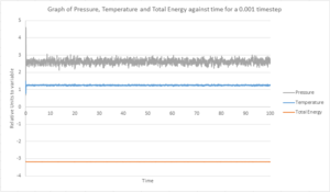
From Fig.3 and Fig. 4, we can see that after the initial spikes in pressure, energy and temperature, the system quickly reaches equilibrium. The equilibrium mean temperature is approximately 1.2554 ± 0.0222, mean pressure is 2.6156 ± 0.1310 and average total energy is -3.1842 ± 0.0007. The ± numbers are standard deviations calculated from the data.

From Fig. 4, it is clear that the system reaches equilibrium very quickly, and is between 0.05 - 1 for temperature and pressure. The total energy reaches equilibrium more rapidly. This is because, as discussed earlier, the total energy of the system must be conserved.

From Fig. 5, it can be seen that the majority of the timesteps trialed reach an average total energy as is expected. 0.015 does, however, not. The most likely reason for this is because the timestep is too large and therefore covers too large a period of actual time. The fluctuations in this timestep are also very large. The largest one which could be used to give acceptable results is a timestep of 0.01. This shows a flat total energy with lower fluctuations compared to 0.015. As the timestep decreases, the fluctuations about a mean value start to decrease too.

JC: Average total energy should not depend on the choice of timestep as it does for 0.01 and 0.0075. 0.0025 and 0.001 give the same average energy and so choosing the larger of these, 0.0025, might be a better choice.

Running Simulations Under Specific Conditions

Temperature and Pressure Control

TASK: Choose 5 temperatures (above the critical temperature $T^{*} = 1.5$ ), and two pressures (you can get a good idea of what a reasonable pressure is in Lennard-Jones units by looking at the average pressure of your simulations from the last section). This gives ten phase points — five temperatures at each pressure. Create 10 copies of npt.in, and modify each to run a simulation at one of your chosen $(p, T)$ points. You should be able to use the results of the previous section to choose a timestep. Submit these ten jobs to the HPC portal.

Temperatures of 1.8, 2.1, 2.4, 2.7 and 3 were chosen and pressures of 2.5 and 5 were used. A timestep of 0.001 was selected so that smaller fluctuations between the temperature and pressure variables would be obtained. This timestep should also allow a good compromise between the value obtained and the 'real time' length of the simulation.

Thermostates and Barostats

TASK: We need to choose $γ$ so that the temperature is correct $T = 𝔗$ if we multiply every velocity $γ$ . We can write two equations:

$E_{K} = \frac{3}{2} N k_{B} T$

$\frac{1}{2} \sum_{i} m_{i} v_{i}^{2} = \frac{3}{2} N k_{B} T$

Solve these to determine $γ$ .

From above:

\frac{1}{2} \sum_{i} m_{i} v_{i}^{2} = \frac{3}{2} N k_{b} T

(6) But

γ

is a co-efficient/ correction for the velocity so target temperature,

τ

, is reached. Hence Eqn. 6 may be re-written as:

\frac{1}{2} \sum_{i} m_{i} γ^{2} v_{i}^{2} = \frac{3}{2} N k_{b} τ

(7) Finally, by combining both Eqn. 6 and Eqn. 7 above:

γ = \sqrt{\frac{τ}{T}}

JC: Correct.

It is also interesting to note that the equipartition function only takes into account kinetic energy and hence why there is no potential term here.

Examining the input script

TASK: Use the manual page to find out the importance of the three numbers 100 1000 100000. How often will values of the temperature, etc., be sampled for the average? How many measurements contribute to the average? Looking to the following line, how much time will you simulate?

100: For every 100 timesteps, use an input value.

1000: To calculate an average value, use an input value 1000 times.

100,000: The simulation will calculate average every 100,000 timesteps.

1000 input values contribute to the average.

100,000 time units will be simulated as a result.

Plotting the Equations of State

TASK: When your simulations have finished, download the log files as before. At the end of the log file, LAMMPS will output the values and errors for the pressure, temperature, and density $(\frac{N}{V})$ . Use software of your choice to plot the density as a function of temperature for both of the pressures that you simulated. Your graph(s) should include error bars in both the x and y directions. You should also include a line corresponding to the density predicted by the ideal gas law at that pressure. Is your simulated density lower or higher? Justify this. Does the discrepancy increase or decrease with pressure?

Plots of the density as a function of temperature were created for the simulations above:

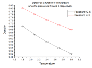
Fig. 6 shows that for a given temperature, a higher pressure means that the system has a higher density. This is intuitive because at a given temperature, there is a constant amount of thermal energy within both systems. Therefore the only variable which can effect the density is the pressure applied to the system. Since the number of particles, $N$ , in the system is constant, the effect due to the increased pressure will be on the volume. By recalling $ρ_{N} = \frac{N}{V}$ , as the volume,( $V$ ) decreases, the density increases. This trend can be followed across the temperature range, but is more pronounced for lower pressures compared to higher ones.

In addition, as the temperature is increased, the density of the substance decreases given a constant pressure. The reason for this is because increasing temperature supplies the system with a larger amount of thermal energy. As a result, there is a greater number of collisions between the fixed number of atoms. This causes an increase in the volume of the system and hence a decrease in the density.

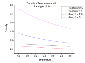
Fig. 7 (above) illustrates that when the system run is analysed with that of the ideal gas law. Some manipulation of the law is first required:

It is well established that for an ideal system:

P V = N k_{b} T

Rearranging yields:

ρ = \frac{N}{V} = \frac{P}{k_{b} T}

Where

ρ

is the density of the system. Note that since reduced terms are used, it can be explicitly stated that

k_{b} = 1

. Hence the final equation is obtained as:

ρ = \frac{P}{T}

(8)

The data shows that if the system was treated ideally, then the density of the system would have been larger. This is because of the assumptions we make when we are using an ideal approximation ^[2]:

1) There are no interactions between any of the particles

2) All the particles are 'points' and do not occupy a volume

3) The system may be treated classically

4) The time it takes for a collision to occur is much larger than the collision time.

If P=2.5 is compared to an ideal and simulated system, the density of the ideal system is larger than that of the simulated system. This is because in an ideal system, at a constant temperature, there is a constant amount of thermal energy applied to the systems. Since in the ideal approximation, we are assuming that there are no interactions, the atoms within the system are likely to pack more closely together and hence the density of the system will be higher. In addition, since 'points' are used, it is significantly a smaller volume is occupied for a given pressure and hence the density will be higher.

JC: Correct, why do the simulation and ideal gas results get closer together at higher temperatures.

Calculating Heat Capacities using Statistical Physics

Heat Capacity Calculation

TASK: As in the last section, you need to run simulations at ten phase points. In this section, we will be in density-temperature $(ρ^{*}, T^{*})$ phase space, rather than pressure-temperature phase space. The two densities required at $0.2$ and $0.8$ , and the temperature range is $2.0, 2.2, 2.4, 2.6, 2.8$ . Plot $C_{V} / V$ as a function of temperature, where $V$ is the volume of the simulation cell, for both of your densities (on the same graph). Is the trend the one you would expect? Attach an example of one of your input scripts to your report.

Extract 1 below shows the example script for the heat capacity where $ρ^{*} = 0.2$ and $T^{*} = 2.0$ have been used. The script has been made by editing the npt.in script:

Extract 1 - Note that this is has edited from the npt.in file provided to meet the needs of the task. ^[1]

### DEFINE SIMULATION BOX GEOMETRY ###
variable D equal 0.2
lattice sc ${D}
region box block 0 15 0 15 0 15
create_box 1 box
create_atoms 1 box

### DEFINE PHYSICAL PROPERTIES OF ATOMS ###
mass 1 1.0
pair_style lj/cut/opt 3.0
pair_coeff 1 1 1.0 1.0
neighbor 2.0 bin

### SPECIFY THE REQUIRED THERMODYNAMIC STATE ###
variable T equal 2.0
variable p equal 0.2
variable timestep equal 0.001

### ASSIGN ATOMIC VELOCITIES ###
velocity all create ${T} 12345 dist gaussian rot yes mom yes

### SPECIFY ENSEMBLE ###
timestep ${timestep}
fix nve all nve

### THERMODYNAMIC OUTPUT CONTROL ###
thermo_style custom time etotal temp press
thermo 10

### RECORD TRAJECTORY ###
dump traj all custom 1000 output-1 id x y z

### SPECIFY TIMESTEP ###

### RUN SIMULATION TO MELT CRYSTAL ###
run 10000
unfix nve
reset_timestep 0

### BRING SYSTEM TO REQUIRED STATE ###
variable tdamp equal ${timestep}*100
variable pdamp equal ${timestep}*1000
fix nvt all nvt temp ${T} ${T} ${tdamp}
run 10000
reset_timestep 0
unfix nvt
fix nve all nve

### MEASURE SYSTEM STATE ###
thermo_style custom step etotal temp press density atoms
variable N equal atoms
variable E equal etotal
variable E2 equal etotal*etotal
variable dens equal density
variable dens2 equal density*density
variable temp equal temp
variable temp2 equal temp*temp
variable press equal press
variable press2 equal press*press
fix aves all ave/time 100 1000 100000 v_dens v_temp v_press v_dens2 v_temp2 v_press2 v_E v_E2
run 100000

variable avedens equal f_aves[1]
variable avetemp equal f_aves[2]
variable avepress equal f_aves[3]
variable errdens equal sqrt(f_aves[4]-f_aves[1]*f_aves[1])
variable errtemp equal sqrt(f_aves[5]-f_aves[2]*f_aves[2])
variable errpress equal sqrt(f_aves[6]-f_aves[3]*f_aves[3])
variable hc equal (${N}*${N})*((f_aves[8]-(f_aves[7]*f_aves[7]))/(f_aves[5]))

print "Density: ${avedens}"
print "Temperature: ${avetemp}"
print "Heat Capacity: ${hc}"

Fig. 8 below illustrates the normalised heat capacity of the system with respect to temperature:

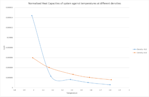
Fig. 8 shows the generalCorrect trend that as temperature increases, for a given density, the heat capacity of the system decreases. If the definition of specific heat capacity is firstly considered; it is the energy required to increase the energy of a system, with unit mass, by 1 K. Hence as T increase, a lower amount of thermal energy needs to be supplied to increase the temperature by 1 K. This is because at high T, there the number of collisions between particles increases and therefore will be able to transfer energy more rapidly and effectively. Consequently, the heat capacity of the system, at constant volume and density, will decrease.

There is an anomalous result for $T = 2.0$ , when $ρ^{*} = 0.2$ . The normalised heat capacity for this value is significantly higher than that of the the other results. It was expected that this value lie below the ρ* = 0.8 curve. Re-running of this specific simulation yielded the same result, so this is not a computational error. The reason for this point could be because when simulations are run computationally, approximations are made and this may have resulted in this point.

Following the trend in Fig. 8 for the points at a higher temperature, it is visible that given a constant temperature, the heat capacity of $ρ^{*} = 0.8$ is higher than that of $ρ^{*} = 0.2$ . Firstly, it is important to recall that the heat capacity on the y-axis of Fig. 8 is $C_{V} / V$ and therefore a volume normalised heat capacity. This means that comparisions between the two densities can be made appropriately. For $ρ^{*} = 0.2$ , there would need to be a larger volume to occupy all the atoms (3375 of them) into a space of the required density. This means that the specific heat capacity of the system would decrease because the particles, although they are more free to move, transfer heat energy less effictively. By contrast, when $ρ^{*} = 0.8$ , a smaller volume is required and the 3375 atoms are more closely packed together. This means that the nearest atom distance is lower and energy is transferred more effectively via collisions. Therefore a lower normalised heat capacity is observed for lower densities.

JC: The trend with density is not about the frequency of collisions. At higher densities there will be more particles in a given volume and hence more energy must be supplied per volume to raise the temperature by 1K.

Structural Properties and the Radial Distribution Function

Simulations in this section

TASK: perform simulations of the Lennard-Jones system in the three phases. When each is complete, download the trajectory and calculate $g (r)$ and $\int g (r) d r$ . Plot the RDFs for the three systems on the same axes, and attach a copy to your report. Discuss qualitatively the differences between the three RDFs, and what this tells you about the structure of the system in each phase. In the solid case, illustrate which lattice sites the first three peaks correspond to. What is the lattice spacing? What is the coordination number for each of the first three peaks?

Values for the density and temperature for the system corresponding to a solid, liquid and vapour phase were chosen based on the work by Hansen and Verlet in Lennard-Jones phase diagrams. ^[3]

Table 2 below shows the variables selected:

**Table 2** Variables used to calculate the radial distribution function
	Solid	Liquid	Vapour
Density	1.2	0.8	0.01
Temperature	1.0	1.0	1.0

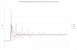
It is first important to firstly consider what Fig. 9 represents; the peaks for each respective state are the nearest neighbour distance from the atom under consideration. It is, therefore, possible to determine the environment with respect to the atom under consideration and simulate what the system may look like.

Comparing the Vapour and Liquid, it can be seen that there is one broad peak for the vapour before falling to zero; whereas with liquid, there is an initial sharp peak at the same distance, but then appears to be a form of sinusoidal exponential decay. The reason why vapour only has one peak at $g (r) = 2.47$ is because a gas has several more degrees of freedom compared to a liquid. This implies that there is more likely to be a lower degree of order within the system. This may help explain why the peak is broad in vapour as there there is no regular spacing thereafter unlike in the liquid, where the atom will still see some order around it.

Comparing the Liquid and Solid radial distribution functions, the solid's function has sharper and less smooth peaks compared to the liquid, which can be explained by the fact that a liquid is more dynamic (it is easier to move atoms in a liquid than in a solid). Since there there are peaks occur approximately every 0.3-0.5 distance units, which shows that the solid has a very regular structure no matter how far the atom under consideration is. However, this is not the case with a liquid and is more interesting. There appears to be a regular degree of order to begin with which then disappears as we move further away from the atom under consideration. In liquids, this atom could form 'atom shells' around it - so the first nearest neighbour peak is the first shell, second peak is the second shell and so forth. It makes sense that as distance between atoms is increased, their interactions decrease and consequently why $g (r)$ decreases as $r$ increases for a liquid.

JC: The liquid has short range order, but no long range order, unlike the solid. The solid has peaks at large r indicating the lattice structure.

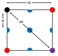
Fig. 10 above shows the three different environments around the black atom in the FCC lattice, and this gives rise to the first three initial peaks in the radial distribution function. The closest atom to the black atom is the blue (denoted (I)), and this will have the lowest $r$ value. Then it is the red and finally in purple; with the purple being the cause of the third peak.

JC: The purple atom is not responsible for the 3rd peak, if you draw the structure in 3D you should be able to spot an atom closer to the black atom than the purple one is. Did you calculate the lattice spacing? You could then have compared the distances to these atoms with the positions of the peaks in g(r).

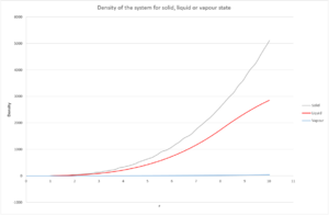
The integral of the radial distribution function is equal to the density of the system. It can be seen from Fig. 11 that this is fairly constant for a gas compared to a solid and liquid.

From the $g (r)$ plot, and the density plot, it is possible to calculate the co-ordination number of the system at each peak. The area under the first peak gives the value of the density at those $r$ values. For example, the first peak lies between $0.8 < r < 1.2$ . By comparing this range to the graph in Fig. 11, it's possible to work out the density. This evaluates to approximately 12. This value also seems like a sound co-ordination number because in an FCC lattice, an atom will have 12 neighbors to it (referring to Fig. 10 where there is only 1 unit cell, the atom has 3 nearest neighbours. Scale this up to 4 and there are 12). By repeating this process for the others, the density of the 2nd peak is 6 and 3rd is approximately 24.

JC: Can you see that there are 6 and 24 atoms responsible for the other peaks from the structure?

Dynamical Properties and the Diffusion Co-efficient

Mean Squared Displacement

TASK: In the D subfolder, there is a file liq.in that will run a simulation at specified density and temperature to calculate the mean squared displacement and velocity autocorrelation function of your system. Run one of these simulations for a vapour, liquid, and solid. TASK: make a plot for each of your simulations (solid, liquid, and gas), showing the mean squared displacement (the "total" MSD) as a function of timestep. Are these as you would expect? Estimate $D$ in each case. Be careful with the units! Repeat this procedure for the MSD data that you were given from the one million atom simulations.

The same conditions as in Table 2 were used in this simulation.

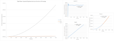
The plots from Fig. 12 below show that the total mean squared displacement is much larger for a vapour than for a solid. This is expected since in a gaseous system, there is more room for movement. In a solid, each atom is 'fixed' in its respective position and hence will only be able to move by very small amounts from that position before returning to it. For gases and liquids, there is a large increase possible because the atoms are not fixed and that of a gas is larger than of a liquid. A reason for this could be that the gas and liquid both follow Brownian motion: for the liquid, since the atoms are closer together, one atom will move a shorter distance compared to that of a gas where atoms are much further apart. The values of D are: D[solid] = 0 (the value for D obtained for a solid is very, very small); D[liquid] = 1.33x10^-4; D[vapour] = 0.0121 area/unit time.

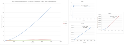
The value for diffusion co-efficient, $D$ , for the solid is expected to remain 0. D[vapour] = 0.006 and D[liquid] = 1.66x10^-4. The calculation shows that the value for the diffusion co-efficient has increased. This is because with one million atoms, there is significantly larger sample taken and so will represent a more accurate value for the system.

JC: Results look good. Why do you think the mean squared displacement graph is not a straight line to begin with, especially for the gas?

Velocity Autocorrelation Function

TASK: In the theoretical section at the beginning, the equation for the evolution of the position of a 1D harmonic oscillator as a function of time was given. Using this, evaluate the normalised velocity autocorrelation function for a 1D harmonic oscillator (it is analytic!):

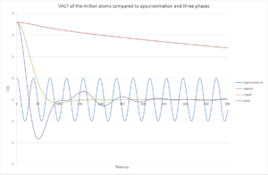
$C (τ) = \frac{\int_{- \infty}^{\infty} v (t) v (t + τ) d t}{\int_{- \infty}^{\infty} v^{2} (t) d t}$

Be sure to show your working in your writeup. On the same graph, with x range 0 to 500, plot $C (τ)$ with $ω = 1 / 2 π$ and the VACFs from your liquid and solid simulations. What do the minima in the VACFs for the liquid and solid system represent? Discuss the origin of the differences between the liquid and solid VACFs. The harmonic oscillator VACF is very different to the Lennard Jones solid and liquid. Why is this? Attach a copy of your plot to your writeup.

The analytical solution for the position of a 1D harmonic oscillator is given by:

x (t) = A \cos (ω t + ϕ)

hence by differentiation, the velocity is obtained:

x^{'} (t) = v (t) = - A ω \sin (ω t + ϕ)

By considering the value at

v (t + τ)

, it can be seen that:

v (t + τ) = - A ω \sin (ω (t + τ) + ϕ)

So the integral becomes

C (τ) = \frac{(A ω)^{2} \int_{- \infty}^{\infty} \sin (ω t + ϕ) \sin (ω (t + τ) + ϕ) d t}{(A ω)^{2} \int_{- \infty}^{\infty} \sin^{2} (ω t + ϕ) d t}

(9)

If we first calculate the denominator of this integral:

(A ω)^{2} \int_{- \infty}^{\infty} \sin^{2} (ω t + ϕ) d t

It is well established that:

\sin^{2} (x) = \frac{1}{2} [1 - \cos 2 x]

Hence it follows that the integral becomes:

\frac{(A ω)^{2}}{2} \int_{- \infty}^{\infty} 1 - \cos (2 ω t + 2 ϕ) d t

This integral may be evaluated as:

[t - \frac{1}{2 ω} \sin (2 ω t + 2 ϕ)]_{- \infty}^{\infty}

(10)

If the numerator is now calculated:

(A ω)^{2} \int_{- \infty}^{\infty} \sin (ω t + ϕ) \sin (ω (t + τ) + ϕ) d t

It is possible to re-write the second sine function as:

\sin (ω (t + τ) + ϕ) = \sin (ω t + ϕ + ω τ)

By using the trig. angle formula:

\sin (G + B) = \sin (G) \cos (B) + \sin (B) \cos (G)

Given that

G = ω t + ϕ

and

B = ω τ

, it can be seen that the integral transforms into:

(A ω)^{2} \int_{- \infty}^{\infty} \sin (ω t + ϕ) [\sin (ω t + ϕ) \cos (ω τ) + \sin (ω τ) \cos (ω t + ϕ)] d t

Which once expanded yields:

(A ω)^{2} \cos (ω τ) \int_{- \infty}^{\infty} \sin^{2} (ω t + ϕ) d t + (A ω)^{2} \sin (ω τ) \int_{- \infty}^{\infty} \sin (ω t + ϕ) \cos (ω t + ϕ) d t

It should be noted that the first integral on the left hand side was previously calculated as the denominator and also yields Eqn. 10 above as the answer.

To calculate the second integral:

(A ω)^{2} \sin (ω τ) \int_{- \infty}^{\infty} \sin (ω t + ϕ) \cos (ω t + ϕ) d t

This integral can be calculated via inspection or substitution:

u (t) = \sin (ω t + ϕ)

\Rightarrow u^{'} (t) = ω \cos (ω t + ϕ)

After applying the substitution, the cosine terms will cancel, leaving (note the limits do not change here):

A^{2} ω \sin (ω τ) \int_{- \infty}^{\infty} u d u

Which are evaluation and re-insertion of

u

:

\frac{1}{2} A^{2} ω \sin (ω τ) [\sin^{2} (ω t + ϕ)]_{- \infty}^{\infty}

By substituting this back into Eqn. 9:

C (τ) = \frac{(A ω)^{2} \cos (ω τ) [t - \frac{1}{2 ω} \sin (2 ω t + 2 ϕ)]_{- \infty}^{\infty} + \frac{1}{2} A^{2} ω \sin (ω τ) [\sin^{2} (ω t + ϕ)]_{- \infty}^{\infty}}{\frac{1}{2} (A ω)^{2} [t - \frac{1}{2 ω} \sin (2 ω t + 2 ϕ)]_{- \infty}^{\infty}}

After evaluating the limits, the solution converges and are left with:

C (τ) = \frac{\frac{1}{2} (A ω)^{2} \cos (ω τ) t}{\frac{1}{2} (A ω)^{2} t}

Which finally yields as the answer:

C (τ) = \cos (ω τ)

(10)

JC: Derivation can be simplified so that no integration is needed. Once you have used the trig angle formula, the sin squared integral cancels with the integral in the denominator and the sin*cos integral must be zero because it is an odd function integrated between limits symmetric about zero.

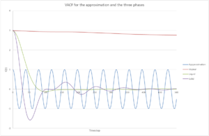
The minima from the VACFs (Fig. 14 above) in the liquid and solid represent that there is a change in velocity, The minima represent that the atom's velocity is changing direction. There are greater number of minima in a solid compared to in a liquid. This is because in a solid FCC lattice, all atoms are fixed in their relative positions and so can only oscillate from this position. In a liquid, this is not true. It is interesting to note that for the solid, the VACF looks very much like an oscillator which has been damped; and hence why an atom is losing velocity over a period of time. This damping may be because when we start the simulation at t=0, the atom has the greatest energy, but then due to various interactions between it and other atoms within the lattice, it is pulled in various directions and hence why the oscillations appear damped.^[4] Here, the solid looks like it would work well with the approximation made because the VACFs are initially of similar magnitudes - so this would be a good approximation at low time periods. The vapour would be a poor choice since it follows no oscillatory velocity.

The VACF is different from the Lennard-Jones solid and liquid because in VACF, it is taken that each atom has an initial velocity.

JC: Which approximation are you talking about? Why is the VACF for the harmonic oscillator different to the simulation? The presence of random collisions in the simulation causes the VACF to decorrelate.

TASK: Use the trapezium rule to approximate the integral under the velocity autocorrelation function for the solid, liquid, and gas, and use these values to estimate $D$ in each case. You should make a plot of the running integral in each case. Are they as you expect? Repeat this procedure for the VACF data that you were given from the one million atom simulations. What do you think is the largest source of error in your estimates of D from the VACF?

Fig. 15 below shows the running trapezium-rule (Eqn. 11) integral and Table 3 shows the total values from use of the trapezium-rule and the calculated D values from the given equation (Eqn. 12)

Eqn. 11 The Trapezium rule in its most basic form:

A r e a = \frac{1}{2} \times w i d t h \times [(1 s t h e i g h t) + 2 (s u m o f o t h e r h e i g h t s)_{n - 1} + (l a s t h e i g h t)_{n}]

Eqn. 12 The difussion co-efficient from the velocity autocorrelation function:^[1]

D = \frac{1}{3} \int_{0}^{\infty} C (τ) d τ

**Table 3** Values from the trapezium rule and values for the diffusion co-efficient.
	Solid	Liquid	Vapour
Trapezium integrals	5.64x10^-4	0.248	21.4
D/ area/unit time	1.88x10^-4	0.0826	7.12

The integral values obtained are of the correct trend (ie vapour> liquid> solid). The reason for this trend is that it is expected that gaseous atoms can retain their velocities for longer without there being a significant decrease (there are few regular interactions). However, for a liquid and solid, there are nearby atoms which cause the velocity to change and therefore have much lower values for the integral. The diffusion co-efficients still follow the same trend as above as expected.

For 1 million atoms:

**Table 4** Values from the trapezium rule and values for the diffusion co-efficient for 1 million atoms.
	Solid	Liquid	Vapour
Trapezium integrals	1.37x10^-4	0.270	9.81
D/ area/unit time	4.55x10^-5	0.0901	3.27

The data for the 1 million atom simulation is lower for both the integral and the diffusion co-efficient. One of the major sources of error comes from the trapezium rule where the integral is not exact and therefore can be an over/ underestimate to the VACF. This can therefore lead to a large error in D.

JC: Calculating the diffusion coefficient using the VACF depends on the integral of the VACF reaching a plateau.

References

↑ ^1.0 ^1.1 ^1.2 https://wiki.ch.ic.ac.uk/wiki/index.php?title=Third_year_simulation_experiment
↑ P. Atkins, J. de Paula; Atkins’ Physical Chemistry; Oxford University Press; Oxford; Ninth Edition; 2009; pp 25-27.
↑ J. Hansen, L. Verlet; Phys. Rev.; 1969; Vol. 184, Issue 1; pp 151-184. DOI: https://doi.org/10.1103/PhysRev.184.151
↑ Democritus: The Velocity Autocorrelation Function.http://www.compsoc.man.ac.uk/~lucky/Democritus/Theory/vaf.html [Accessed 26/01/2017]

[Wiki_task_page-1] 1.0 ^1.1 ^1.2 https://wiki.ch.ic.ac.uk/wiki/index.php?title=Third_year_simulation_experiment

[2] P. Atkins, J. de Paula; Atkins’ Physical Chemistry; Oxford University Press; Oxford; Ninth Edition; 2009; pp 25-27.

[3] J. Hansen, L. Verlet; Phys. Rev.; 1969; Vol. 184, Issue 1; pp 151-184. DOI: https://doi.org/10.1103/PhysRev.184.151

[4] Democritus: The Velocity Autocorrelation Function.http://www.compsoc.man.ac.uk/~lucky/Democritus/Theory/vaf.html [Accessed 26/01/2017]

[1]

[2]

[3]

[4]

Liquid Simulations[1]

Introduction to Molecular Dynamics

The Classical Particle Approximation

Atomic Forces

Periodic Boundary Conditions

Reduced Units

Equilibration

Output of the first simulation

Creating the Simulation box

Setting the Properties of the atoms

Running the Simulation

Checking Equilibration

Running Simulations Under Specific Conditions

Temperature and Pressure Control

Thermostates and Barostats

Examining the input script

Plotting the Equations of State

Calculating Heat Capacities using Statistical Physics

Heat Capacity Calculation

Structural Properties and the Radial Distribution Function

Simulations in this section

Dynamical Properties and the Diffusion Co-efficient

Mean Squared Displacement

Velocity Autocorrelation Function

References

Liquid Simulations^[1]