Talk:LH3115-Liquidsimulations
This is a nice report Lorenz! Although there were minor things in the understanding, you write really well. Keep this sort of style for your thesis :) Mark: 68/100
Tasks from the lab script
Tasks Introduction to molecular dynamics simulation
TASK: Open the file HO.xls. In it, the velocity-Verlet algorithm is used to model the behaviour of a classical harmonic oscillator. Complete the three columns "ANALYTICAL", "ERROR", and "ENERGY": "ANALYTICAL" should contain the value of the classical solution for the position at time t, "ERROR" should contain the absolute difference between "ANALYTICAL" and the velocity-Verlet solution (i.e. ERROR should always be positive -- make sure you leave the half step rows blank!), and "ENERGY" should contain the total energy of the oscillator for the velocity-Verlet solution. Remember that the position of a classical harmonic oscillator is given by x\left(t\right) = A\cos\left(\omega t + \phi\right) (the values of A, omega, and phi are worked out for you in the sheet).

TASK: For the default timestep value, 0.1, estimate the positions of the maxima in the ERROR column as a function of time. Make a plot showing these values as a function of time, and fit an appropriate function to the data.
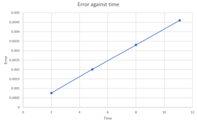
TASK: Experiment with different values of the timestep. What sort of a timestep do you need to use to ensure that the total energy does not change by more than 1% over the course of your "simulation"? Why do you think it is important to monitor the total energy of a physical system when modelling its behaviour numerically?
 |
 |
0.2 is the maximum timestep allowed. It is important to monitor the energy of a system in order for calculations to be accurate and to know when what happens. Tick
TASK: For a single Lennard-Jones interaction
Tasks Equilibration
TASK: Why do you think giving atoms random starting coordinates causes problems in simulations? Hint: what happens if two atoms happen to be generated close together?:
The problem with this would be that if the molecules were to generate in the same space the very close to each other, the simulation would blow up as to much repulsion force is simulated. Tick, good
TASK: Satisfy yourself that this lattice spacing corresponds to a number density of lattice points of 0.8. Consider instead a face-centred cubic lattice with a lattice point number density of 1.2. What is the side length of the cubic unit cell?
In a simple cubic unit cell there is one atom in the middle of the cube, therefore: Tick
Using the face centered cubic unit cell the number of particles per unit cell is 3 and changing the density to 1.2, the edge of the cube is: The number of atoms per unit cell for fcc is 4.. not quite right!
TASK: Consider again the face-centred cubic lattice from the previous task. How many atoms would be created by the create_atoms command if you had defined that lattice instead?
The unit cell has 3 lattice points in the fcc, therefore using the density of 1.2 and the side length of 1.3572, the number of atoms would be 3000. As the code adapts to the size of the unit cell we defined. again fcc has 4 atoms in its unit cell
TASK: Given that we are specifying x_i(0) and v_i(0), which integration algorithm are we going to use?
The velocity verlet algorithm, as it requires to know the starting velocity and starting position of each atom. Tick
TASK: Using the LAMMPS manual, find the purpose of the following commands in the input script:
mass 1 1.0
pair_style lj/cut 3.0
pair_coeff * * 1.0 1.0
The mass define the atom type first and the second value defines the mass of said atom type.
The pair style defines the when pair wise interactions take place. Here the cutoff is at a distance of 3 between two particles i j. It also specifies that the Lenard-Jones potential is used for calculating the pair wise interactions:
with
The coefficients for the pair style are given by the command pair_coeff, so here it is 1 for each atom involved in the interaction
The asterisk is used to define the atom type while the numbers set the coefficient values.
TASK: Look at the lines below.
.### SPECIFY TIMESTEP ###
variable timestep equal 0.001
variable n_steps equal floor(100/${timestep})
timestep ${timestep}
.### RUN SIMULATION ######
run ${n_steps}
run 100000
TASK:The second line (starting "variable timestep...") tells LAMMPS that if it encounters the text ${timestep} on a subsequent line, it should replace it by the value given. In this case, the value ${timestep} is always replaced by 0.001. In light of this, what do you think the purpose of these lines is? Why not just write:
timestep 0.001
run 100000
By writing it the way it is written we can change the value of the timestep and that will automatically change all necessary values for us. We assign a variable which makes it easier to change the settings later on.
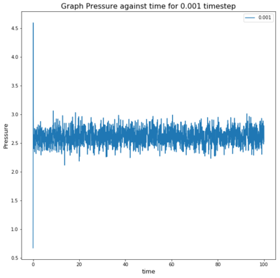
TASK: make plots of the energy, temperature, and pressure, against time for the 0.001 time step experiment (attach a picture to your report). Does the simulation reach equilibrium? How long does this take? When you have done this, make a single plot which shows the energy versus time for all of the time steps (again, attach a picture to your report). Choosing a time step is a balancing act: the shorter the time step, the more accurately the results of your simulation will reflect the physical reality; short time steps, however, mean that the same number of simulation steps cover a shorter amount of actual time, and this is very unhelpful if the process you want to study requires observation over a long time. Of the five time steps that you used, which is the largest to give acceptable results? Which one of the five is a particularly bad choice? Why?
 |
 |

|
The simulation reaches equilibrium almost instantly, as seen in all three graphs.

In this graph one can see that all time step values except 0.015 reach equilibrium, so it would be a very bad choice as a time step. This means anything above 0.01 is a very bad choice as the energy keeps increasing as seen in the graph. The highest acceptable value for the time step is 0.0025 as it is the highest value time step, which still has the lowest energy equilibrium. As the lowest energy is the most stable configuration, therefore the simulation value with the lowest energy is the most accurate. Given that the 0.0025 time step is the same energy as the 0.001 it is still accurate. Tick
Tasks:Running simulations under specific conditions
TASK: We need to choose γ so that the temperature is correct T = target T if we multiply every velocity γ. We can write two equations:
Tick, good
TASK: Use the manual page to find out the importance of the three numbers 100 1000 100000. How often will values of the temperature, etc., be sampled for the average? How many measurements contribute to the average? Looking to the following line, how much time will you simulate?
The 100000 is nfreq in the code which determines that every 100000 timestep an average is taken. Nevery is 100 and says that every 100 values contribute to an recorded average. The 1000 is Nrepeat and determines how many of the Nevery averages contribute to the overall average. Note that the first two values multiplied do not exceed 100000 and that 100000 is a multiple of 100. Tick
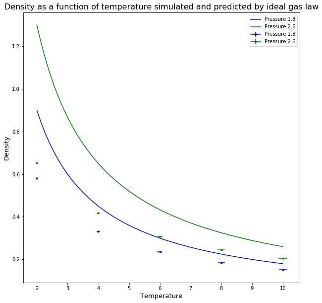
TASK: When your simulations have finished, download the log files as before. At the end of the log file, LAMMPS will output the values and errors for the pressure, temperature, and density. Use software of your choice to plot the density as a function of temperature for both of the pressures that you simulated. Your graph(s) should include error bars in both the x and y directions. You should also include a line corresponding to the density predicted by the ideal gas law at that pressure. Is your simulated density lower or higher? Justify this. Does the discrepancy increase or decrease with pressure?
The graph show both simulated and data predicted by the ideal gas law. The density for both systems decreases as the temperature increases as the particles move more and have more energy. The density of the predicted values using the ideal gas law are higher than the simulated values, this is due to the fact that the ideal gas law ignores interactions between particles, however the particles in the simulation use the Lenard-Jones potential, there is a repulsion term therefore the particles spread out more, therefore the density is less. With increased pressure the difference between simulated and predicted increases, as the repulsion term becomes greater the closer the particles get, while the ideal gas law doesn't take into account the new proximity of the particles.Tick, what about at high T?
Tasks:Calculating heat capacities using statistical physics
TASK: As in the last section, you need to run simulations at ten phase points. In this section, we will be in density-temperature (p*, T*) phase space, rather than pressure-temperature phase space. The two densities required at 0.2 and 0.8, and the temperature range is 2.0, 2.2, 2.4, 2.6, 2.8. Plot Cv/V as a function of temperature, where V is the volume of the simulation cell, for both of your densities (on the same graph). Is the trend the one you would expect? Attach an example of one of your input scripts to your report
The higher the density the more particles are in the same volume. More particles mean more energy levels and more connections between particles, therefore the heat capacity is higher, see equation:
This should be a proportionality not an equality!
However as we increase the Temperature of the system the heatcapacity should increase as more energy levels are now accessible. But as seen with the higher pressure it starts going down. This trend could occur due to the increased density of states in the higher density simulation. With increasing density of states the lower energy levels go closer together while the higher energy levels have greater spacing. So the greater the temperature the more difficult it is to access the higher energy for higher density systems than lower density systems. So for a similar varience in energy the temperature increases so according to the heat capacity equation the heat capacity decreases. Not fully right, as temperature is higher you could have access to more degrees of freedom (something we may see in melting) and this could increase the heat cap (think equipartition theory). Although, how easy is it to heat a hot thing with the same DOS? If we increase DOS, this should make it easier for the higher states to be populated
Attached input script of heat capacity
|### DEFINE SIMULATION BOX GEOMETRY ###
|variable dens equal 0.8
|lattice sc ${dens}
|region box block 0 15 0 15 0 15
|create_box 1 box
|create_atoms 1 box
|(### DEFINE PHYSICAL PROPERTIES OF ATOMS ###
|mass 1 1.0
|pair_style lj/cut/opt 3.0
|pair_coeff 1 1 1.0 1.0
|neighbor 2.0 bin
|### SPECIFY THE REQUIRED THERMODYNAMIC STATE ###
|variable T equal 2.0
|variable timestep equal 0.0025
|### ASSIGN ATOMIC VELOCITIES ###
|velocity all create ${T} 12345 dist gaussian rot yes mom yes
|### SPECIFY ENSEMBLE ###
|timestep ${timestep}
|fix nve all nve
|### THERMODYNAMIC OUTPUT CONTROL ###
|thermo_style custom time etotal temp press
|thermo 10
|### RECORD TRAJECTORY ###
|dump traj all custom 1000 output-1 id x y z
|### SPECIFY TIMESTEP ###
|### RUN SIMULATION TO MELT CRYSTAL ###
|run 10000
|reset_timestep 0
|unfix nve
|### BRING SYSTEM TO REQUIRED STATE ###
|variable tdamp equal ${timestep}*100
|fix nvt all nvt temp ${T} ${T} ${tdamp}
|run 10000
|reset_timestep 0
|### MEASURE SYSTEM STATE ###
|thermo_style custom atoms etotal temp vol
|variable temp equal temp
|variable temp2 equal temp*temp
|variable volume equal vol
|variable atoms equal atoms
|variable atoms2 equal atoms*atoms
|variable etotal equal etotal
|variable etotal2 equal etotal*etotal
|fix aves all ave/time 100 1000 100000 v_temp v_temp2 v_etotal v_etotal2 v_atoms2
|run 100000
|variable avetemp equal f_aves[1]
|variable aveetotal equal f_aves[3]
|variable aveetotal2 equal f_aves[4]
|variable aveatoms2 equal f_aves[5]
|variable avetemp2 equal f_aves[2]
|print "Averages"
|print "--------"
|print "Temperature: ${avetemp}"
|print "Temperature2: ${avetemp2}"
|print "aveetotal: ${aveetotal}"
|print "aveetotal2: ${aveetotal2}"
|print "atoms: ${atoms}"
|print "volume: ${volume}"
Tasks:Structural properties and the radial distribution function
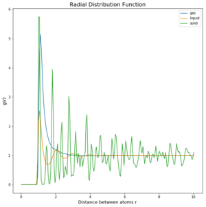
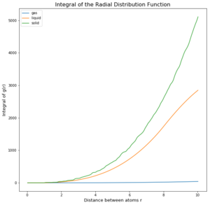
TASK: perform simulations of the Lennard-Jones system in the three phases. When each is complete, download the trajectory and calculate g(r) and integral of g(r). Plot the RDFs for the three systems on the same axes, and attach a copy to your report. Discuss qualitatively the differences between the three RDFs, and what this tells you about the structure of the system in each phase. In the solid case, illustrate which lattice sites the first three peaks correspond to. What is the lattice spacing? What is the coordination number for each of the first three peaks?
 |
 |
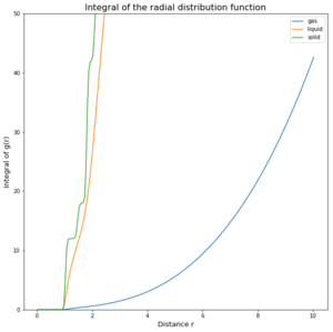 |
The difference of the phases and the density of them can be seen in the 3 graphs (figures 4 to 6) above. In the integrated RDF graph, the gas value is considerably lower than the corresponding liquid and solid values. It is also the first to reach 1 in the RDF graph which means that the local average density at that distance is the same as average density of the system. This makes sense as gases spread out fastest. So at a distance of 3.4 nm, the number of atoms around is approximately 40 compared to the almost 3000 particles in a liquid at the same distance. (fcc atoms) also I would say this is more a measure of uniformity in each of the phases rather than local dens. What does g(r) = 1 mean?
In the RDF graph the liquid reaches 1 at a very short distance, which means again that the local average density equals the average density at that distance. The liquid initially switches between regions of high and low local densities before reaching 1, this could be explained by the fact that most particles aim to get to the optimal distance with each other and therefore these distances will have a greater probability of being populated. Wouldn't say this, would say those initial peaks are solvation shells Because the atoms at that distance will have repulsion as well, there will be less particles in the proximity of high density probability distances creating low density probability distances resulting in this oscillator like shape. Due to particle movement in liquids, at a certain distance the attraction force of one particle is too small to affect the other atoms.
Solids however behave differently, as they are fixed and have minimal movement of atoms. In case of a crystal they even have a defined structure as seen in the radial distribution function graph. There are clear distances at which the local density of particles is high and close to the particle observed is even 0. The solid also averages out and approaches 1 at infinty as at long distances due to the movement of all atoms, the density probability averages out. The first 3 peaks belong to the face centered cubic lattice, the spacing between the first 2 peaks is 0.45 in reduced units or 0.153 nm and 0.35 in reduced units or 0.119 nm for the 2nd and 3rd peak. By looking at the integration of the solid RDF, one can see that the for the first peak the coordination number is 12, 6 for the second and 24 for the 3rd(12,18 and 42 respective integration values). These values are accurate as that is what we predict with a fcc lattice. Tick
Tasks: Dynamical properties and the diffusion coefficient
TASK: In the D subfolder, there is a file liq.in that will run a simulation at specified density and temperature to calculate the mean squared displacement and velocity autocorrelation function of your system. Run one of these simulations for a vapour, liquid, and solid. You have also been given some simulated data from much larger systems (approximately one million atoms). You will need these files later.
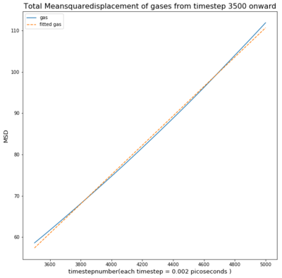
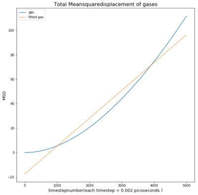
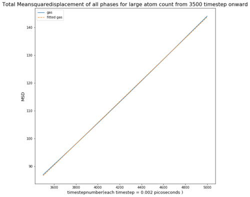
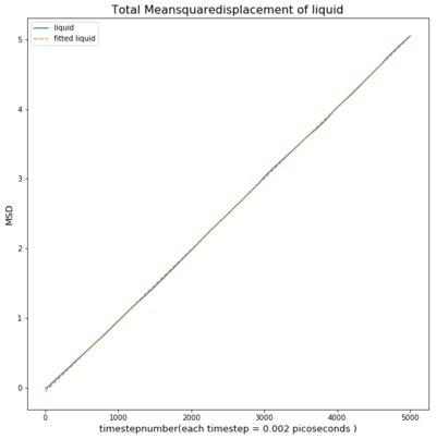
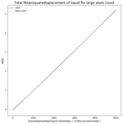
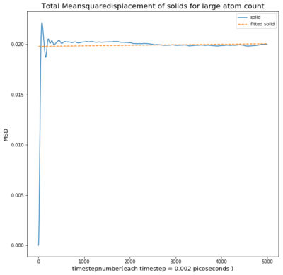
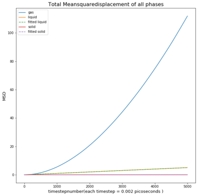
TASK: make a plot for each of your simulations (solid, liquid, and gas), showing the mean squared displacement (the "total" MSD) as a function of timestep. Are these as you would expect? Estimate D in each case. Be careful with the units! Repeat this procedure for the MSD data that you were given from the one million atom simulations.
The Mean Squared Displacement of gases is shown above with the fitted graphs shown. The range for the fitted functions was chosen in the linear region.
 |
 |
 |
 |
 |
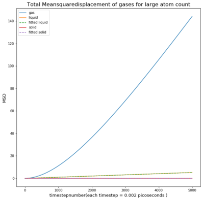 |
As seen in the graph for all phases the msd is highest for gases as they fill out the space they occupy. This means the particle will move away quickly from the reference point, causing a small deviation time.
The liquid has a much smaller msd and follows a linear trend from the beginning
The solid however has a sharp spike at the beginning and settling at an almost constant value.
By calculating Tick
The results of the calculations are given below:

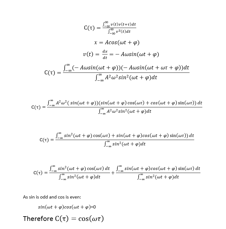
TASK: In the theoretical section at the beginning, the equation for the evolution of the position of a 1D harmonic oscillator as a function of time was given. Using this, evaluate the normalised velocity autocorrelation function for a 1D harmonic oscillator (it is analytic!):

In the graph one can see that all atoms start of with their maximum, however they have different rates of decay toward and their respective minimums. The gas phase just slowly decays in contrast to the other phases and the harmonic oscillator. This can be explained by how the particles interact. Gases spread out and have only weak attraction forces. Therefore the time it takes them to become uncorrelated is very long as no collisions cause the atoms only to slowly change there initial velocities. Think about collisions
Liquids however reach there minimum very quickly and then reach the . One reason could be that the atoms of the liquid do have attractive forces causing them initially to collide which decreases their momentary velocity as kinetic energy is converted to potential. After that initial collision the movements of the atoms is very randomized and therefore quickly reaches .
Solid atoms have fixed defined places within their lattice, so they initially have a high velocity to reach the most stable configuration and oscillate around that spot. This is reflected in the graph above as the solid VCAF oscillates around . Like the liquid it reaches it's minimum first and then decays towards . Solids should therefore show high degrees of correlation?
TASK: Use the trapezium rule to approximate the integral under the velocity autocorrelation function for the solid, liquid, and gas, and use these values to estimate D in each case. You should make a plot of the running integral in each case. Are they as you expect? Repeat this procedure for the VACF data that you were given from the one million atom simulations. What do you think is the largest source of error in your estimates of D from the VACF?
 |
 |

|
 |
 |

|
The trapezium rule was used evaluate the integral in the formula for the diffusion coefficient.

As seen by the coefficients calculated from the VACF, the difference between the diffusion coefficient is already very accurate with a small atom count. However there are clear differences in the liquid case that suggests for more complicated systems a larger atom count is needed. The biggest source of error is the trapezium rule, especially with small numbers as there is not enough averaging. The general trend is as expected that the gaseous running integral is getting bigger but at a slower rate, with each time step, as the VCAF graph approaches . Tick
For the liquid running integral the initial rise comes from the falling from the maximum, the small fall in the integral is explained when the VACF becomes negative, but then it approaches a maximum, as the VACF graph goes to
Due to the constant oscillation in the solid VACF, the corresponding integral approaches 0.
Report
Abstract
Try to develop more of the underlying theme in your abstract - here we explore the properties of phase and dynamics in such systems. Additionally, see the wood for the trees - the fundamental purpose for the calculation of D was not to show that more particles provides a better evaluation of D, it was to show you more a more accurate picture on how D changes with phase.
The conducted simulations show how liquids, solids and gases behave on different conditions. It compares the effectiveness of different assumptions and uses them to calculate properties like heat capacity or density. Using Mean Squared Displacement and Velocity Auto Correlation Functions, the diffusion coefficient was calculated and the necessity of greater particle numbers in simulations was evaluated.
Introduction
Nice - hot topic! Climate. Good intro Lorenz!
Liquids govern the way life on earth works and often their unique behaviors and special features enable life as we know. The unique case of water that makes its solid form less dense than the liquid phase prevents the oceans from freezing. Water is also responsible for keeping the climate as stable as possible due to its high heatcapacity and its density. The ocean regulates the climate by streams where warm water travels towards the poles where it is cooled and sinks and it then returns by lower streams back to place it came from[1]. One way to study these massive systems is by simulating the behavior said systems and analyse them correctly. Therefore one must choose the correct parameter and make the right assumption to learn more about these phenomenons. This labs aims to provide an insight to why liquids (also gases and solids) behave the way they do. It analyses and evaluates heat capacity, diffusion and energy, to provide a first glance at phase behavior and simulations.
Method
All the simulations done in this experiment were run by the high performance computing system from Imperial College London. The provided instruction melt_crystal.in by the lab script was changed in respect to the time step:0.001 s, 0.0025 s, 0.0075 s, 0.01 s, 0.015 s. For all instructions reduced units for argon were used.
A simple cubic lattice with a number density of 0.8 was used in order to specify the location of the atoms, so the simulation wouldn't generate unfeasible energies, in case two atoms are generated in the same space. The lattice spacing was 0.3662548 nm in all 3 Cartesian directions. All atoms created had a mass of 1 and used the Lenard_Jones potential for inter-nuclear forces. The cut off distance for the interactions was 1.02 nm. All pair coefficients were set to 1. The pair wise interactions and mass were not changed in the other simulation instructions. The Temperature was set to 0.0125 K. To analyse the simulation a program called VMD was used. Tick Another simulation was set up in an NPT ensemble using the npt.in file provided in the lab script, 10 simulations were run using the pressures 1.8 and 2.6 at the reduced temperatures 2, 4, 6, 8, 10.The time step chosen for this was 0.0025 as it was the highest acceptable value for which the energy stayed the same from the tests taken.
The next part of the experiment the heat capacity of the system was calculated changing the original npt file from an npt ensemble to an nve ensemble. The densities used were 0.2 and 0.8 at the temperatures in reduced units of 2, 2.2, 2.4, 2.6, 2.8. The input file can be found in the appendix.Tick
The radial distribution function was simulated using the input file from the script and the conditions for the phases were chosen using a phase diagram.[2] The densities chosen were in reduced units 0.05, 0.8 and 1.2. For the temperature 0.5 for gas and solid was used while 1.2 for the liquid was used. A simple cubic for generating the lattice was used for both gas and liquid simulations. For the the solid a face centered cubic was chosen as this is more closely packed. Tick
For the mean squared displacement and the velocity auto correlation function the same parameters for temperature and pressure were used. The instruction file template was provided in the lab script.Tick
Results and Discussion

First the importance of the right time step was analysed by plotting it against total energy. The total energy against time steps graphs show a clear trend. One can see that all time step values except 0.015 reach equilibrium, so it would be a very bad choice as a time step because of changing energies, the simulation results will be incoherent. The highest acceptable value for the time step is 0.0025 as it is the highest value time step, which still has the lowest energy equilibrium. As the lowest energy is the most stable configuration, therefore the simulation value with the lowest energy is the most accurate. Given that the 0.0025 time step is the same energy as the 0.001 it is still accurate and there is no clear difference in noise between the two. Timestep is a given - the timestep should be an accurate representation of the system. If it's too small, you waste your own time, the reader doesn't care ;-)

The extend gram to which density is affected by change in phase was looked at next. The graph shows both the simulated data and the data predicted by the ideal gas law. The density for both systems decreases as the temperature increases, as the particles move more and have more energy. The density of the predicted values using the ideal gas law are higher than the simulated values, this is due to the fact that the ideal gas law ignores interactions between particles, however the particles in the simulation use the Lenard-Jones potential, so there is a repulsion term. Therefore the particles spread out more, which means that the density is less. With increased pressure the difference between simulated and predicted increases, as the repulsion term becomes greater the closer the particles get, while the ideal gas law doesn't take into account the new proximity of the particles.Tick
The Radial Distribution Function was analysed to determine how atoms arrange during the simulation. The difference of the phases and the density of them can be seen in the 3 graphs (figures 4 to 6) above. In the integrated RDF graph, the gas value is considerably lower than the corresponding liquid and solid values. It is also the first to reach 1 in the RDF graph which means that the local average density at that distance is the same as average density of the system. This makes sense as gases spread out fastest. So at a distance of 3.4 nm, the number of atoms around is approximately 40 compared to the almost 3000 particles in a liquid at the same distance.Not the write atom counting for fcc In the RDF graph the liquid reaches 1 at a very short distance, which means again that the local average density equals the average density at that distance. The liquid initially switches between regions of high and low local densities before reaching 1, this could be explained by the fact that most particles aim to get to the optimal distance with each other and therefore these distances will have a greater probability of being populated. Because the atoms at that distance will have repulsion as well, there will be less particles in the proximity of high density probability distances creating low density probability distances resulting in this oscillator like shape. Due to particle movement in liquids, at a certain distance the attraction force of one particle is too small to affect the other atoms. Tick
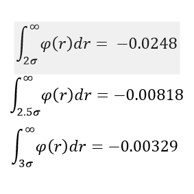
Solids however behave differently, as they are fixed and have minimal movement of atoms. In case of a crystal they even have a defined structure as seen in the radial distribution function graph. There are clear distances at which the local density of particles is high and close to the particle observed is even 0. The solid also averages out and approaches 1 at infinty as at long distances due to the movement of all atoms, the density probability averages out.Tick The first 3 peaks belong to the face centered cubic lattice, the spacing between the first 2 peaks is 0.45 in reduced units or 0.153 nm and 0.35 in reduced units or 0.119 nm for the 2nd and 3rd peak. By looking at the integration of the solid RDF, one can see that the for the first peak the coordination number is 12, 6 for the second and 24 for the 3rd(12,18 and 42 respective integration values). These values are accurate as that is what we predict with a fcc lattice.Tick
 |
 |
The Mean squared displacement was investigated next, in order to obtain the diffusion coefficent.
As seen in the graph for all phases the msd is highest for gases as they fill out the space they occupy. This means the particle will move away quickly from the reference point, causing a small deviation time.
The liquid has a much smaller msd and follows a linear trend from the beginning
The solid however has a sharp spike at the beginning and settling at an almost constant value.
By calculating Tick, if you plotted log-log, why?
The results of the calculations are given below:

Comparing both graphs shows that the large atom count especially in case of the liquid produces a similar diffusion coefficient compared to the smaller atom count.

The Harmonic Oscillator in figure 14 is given by
In the graph (figure 10) one can see the Velocity Auto Correlation Function of all phases. One can observe that all atoms start of at their maximum, however they have different rates of decay toward and their respective minimums.Tick The gas phase just slowly decays in contrast to the other phases and the harmonic oscillator. This can be explained by how the particles interact. Gases spread out and have only weak attraction forces. Therefore the time it takes them to become uncorrelated is very long as no collisions cause the atoms only to slowly change there initial velocities. Tick
Liquids however reach there minimum very quickly and then reach the . One reason could be that the atoms of the liquid do have attractive forces causing them initially to collide which decreases their momentary velocity as kinetic energy is converted to potential. After that initial collision the movements of the atoms is very randomized and therefore quickly reaches .
Solid atoms have fixed defined places within their lattice, so they initially have a high velocity to reach the most stable configuration and oscillate around that spot. This is reflected in the graph above as the solid VCAF oscillates around . Like the liquid it reaches it's minimum first and then decays towards .Tick
 |
 |
 |
The trapezium rule was used evaluate the integral in the formula for the diffusion coefficient.

As seen by the coefficients calculated from the VACF (figure 14), the difference between the diffusion coefficient is already very accurate with a small atom count. However there are clear differences in the liquid case that suggests for more complicated systems a larger atom count is needed. The biggest source of error is the trapezium rule, especially with small numbers as there is not enough averaging. The general trend is as expected that the gaseous running integral is getting bigger but at a slower rate, with each time step, as the VCAF graph approaches .Tick
For the liquid running integral the initial rise comes from the falling from the maximum, the small fall in the integral is explained when the VACF becomes negative, but then it approaches a maximum, as the VACF graph goes to
Due to the constant oscillation in the solid VACF, the corresponding integral approaches 0.Tick
Conclusion
Nice conclusion
The liquid simulation experiment was meant to analyse how different phases act in different situations and how these changes can be characterized. The experiment provides a foundation to how simulations work and how they can be used to obtain almost all information about a liquid. It was found that in order to have a accurate simulation the choice in time step is important. The fundamental difference of the phases was characterized and how they diffuse under ideal conditions was recorded. However the experiment is not reflective on what happen in a real system as outside effects, impurities and different atomic masses can have big effects upon the way the particles behave. The experiment has provides a lot of new application methods, for example analyzing how a liquid with different atoms behaves and how it arranges itself to become a solid crystal. It is also possible to analyze at what point the formation of the crystal occurs or whether one can force a different crystal structure compared to the usual one.
Appendix
references
Cite error: <ref> tag with name "Water" defined in <references> is not used in prior text.
