Talk:Jd2615 comp liq

3=Report=

Not a bad attempt Josh! You've put in a lot of hardwork and you can see it. I think you need to work on seeing the wood for the trees. Don't get too bogged down with rudimentary technicalities - look for the bigger picture. You also miscalculated a few things - have a look through! Mark: 63/100

Abstract

Good abstract but pick and choose what you expect is the important info... timestep is a given. Also units? This experiment investigated the dynamic properties of simulated matter in different states by using the LAMMPS program. The timestep found that the most accurate timestep with the most sensible computing time was 0.0025. The comparison of the lennard-Jones potential to the Ideal Gas Law found that the density of the ideal gas system is always higher the density of the Lennard-Jones system which is attributed to the repulsive term in the Lennard-Jones equation which results in a distribution of particles in a system that tries to reduce unfavorable interactions. Both the Lennard-Jones system and the Ideal gas Law reduced in density as temperature increased from 1.5 to 9.5 (reduced units). The heat-capacity of two systems separated by different densities (0.2 , 0.8) found that as temperature increased from 2.0 to 2.8 (reduced units), the heat capacity decreased. The higher density (0.8) system has a higher heat capacity throughout than the lower density system (0.2). The radial distribution functions solidified the hypothesis that solids have a regular structure, liquids have more motion and are free to move, but may contain microstructures (fluid shells) and liquids have very little ordered structure. For all experiments concerning the diffusion coefficient, it was found that the solid has extremely low diffusion coefficient (roughly 0.2), the liquid has intermediate diffusion coefficient (roughly 0.5) and gas has very high coefficient (roughly 1).

Introduction and Aims

Not bad, but you need to deliver more purpose. Why are we studying the dynamics and phase behaviour of these systems? Why are you talking about water (and don't say because I told you to do so :p) Liquid dynamics has been the interest of scientists for years, especially the dynamic of water. One of the most vital compounds for living organisms, water's properties do not fit the trend when compared to other liquids of similar mass. The ability of water to reduce density on freezing allowing it to float, providing protection for sea creatures in arctic conditions. The high surface tension of water, which provides the necessary forces required for transpiration in plants, the water evaporates from the stigmata in the leaves, drawing water up the xylem and, more importantly from the soil. The universal solvent that cells depend on to suspend the vital compounds of life. The beautiful fractal symmetry that has inspired both scientist and artist alike. Indeed, it has.

Snowflake: from http://www.snowcrystals.com/photos/i0113a331A.jpg

The extraordinary properties of water always feed down to an individual concept, that is the Hydrogen Bond. The pair of hydrogen atoms and lone pairs allow water to bond with it's neighbors in an assortment of ways, depending on the physical conditions that they are in. Research by Pettersson, Lars Gunnar Moody Henchman, Richard Humfry Nilsson, Anders, reiterated the lack of understanding around water, especially the dynamics of the hydrogen bond when exposed to ionic environments. Tick

With the inspiration of water, this experiment will use computational techniques to simulate the dynamics of different states of matter. By simulating groups of simple single point masses, with defined volume, this experiment shall seek out how density of systems varies to the ideal gas states. "single point masses, with defined volume"?? The heat capacity as different densities shall be investigated in order to understand the how a system changes it's ability assimilate energy at different temperatures. Particles can be assumed to hard spheres according to Lennard-Jones system, so each particle can influence the dynamic gram of its neighbours. This investigation shall explore this dynamic by mapping out the general distribution about a central atom using Radial Distribution Functions and investigate how each particle's velocity and displacement affects the velocity and displacement of another using the Velocity Autocorrelation function.

Water's method of 'diffusion' is so vital to chemical and biological processes that it carries it's own name- Osmosis. The diffusion of any system is important to understand, so this experiment shall explore the diffusion coefficients of each state of matter by integrating Velocity Autocorrelation functions and comparing these values with other data acquired from other sources, like taking the gradient of the Mean squared displacement of each state. is the D of water fast or slow relative to other liquids?

Methods

The simulations for this experiment were produced using LAMMPS. For the majority of the simulations a simple cubic lattice with 0.8 unit volume were created as a starting formation of particles before the initiation of the simulation. The lattice spacing in each coordinate direction (x,y,z) were all 1.07722. The pairwise interactions were simulated via Lennard-Jones potential analysis:

$u(r)=4ϵ[(\frac{\sigma }{r}{)}^{12}-(\frac{\sigma }{r}{)}^6]$

Which can be determined by LAMMPS with the following code: 'pair_style lj/cut 3.0 with 'pair_coeff * * 1.0 1.0'. We don't talk about specific syntax in computational methods.. we use phraseology like "a Lennard-Jones forcefield was chosen with a cutoff of 3A and sig/eps = 1." The 'cut' determining the distance r to which the simulation will run and the 'pair_coeff' determines that all particles are included (* *) and the coefficients $ϵ$ and $\sigma$ are both 1 (1.0 1.0).

The equilibration to determine the timestep with the most accuracy balanced with reasonable simulation time was achieved through simulation plots of energy, temperature and pressure of a 1000 atom system with different timesteps. The timesteps used are 0.001, 0.01, 0.015, 0.0025 and 0.0075. This isn't really necessary - you chose the best timestep. You MUST choose an accurate timestep but if the timestep you choose is too small, what's it to the reader that you wasted your own time?

Comparative analysis of the Lennard-Jones system with the ideal gas system was achieved by running simulations of 5 different temperatures (1.5, 3.5, 5.5, 7.5, 9.5 reduced units) at two different pressures (2 and 3 reduced units) then plotting density values of the Lennard-Jones system against density values of the ideal gas law.

The heat capacity of the system is calculated via the following equation:

$C_v=N^2\frac{<E^2>-<E{>}^2}{k_B{T}^2}$

Where $<E^2>-<E{>}^2$ was the variance of energy. The variance can be calculated by simulating the melting of a system within the NVT ensemble with 5 different temperatures (2.0, 2.2, 2.4, 2.6 and 2.8 reduced units) at 2 different density (0.2 and 0.8 reduced units). The energy at each condition was plotted the $<E^2>$ and $<E{>}^2$ are provided to calculate the heat capacity. Tick

The Radial Distribution Function (RDF) was produced by simulating liquid, gas and solid states by varying the temperatures densities corresponding to specific physical states (i.e. gas: T = 1, D = 0.3, Solid: T=0.4, D=1.5, Liquid: T =1.2, D=0.8). The trajectories of each simulation were uploaded to LAMMPS where the RDF and the integral of the RDF are plotted. Tick

The diffusion coefficient was calculated using the gradient of mass squared displacement via the following equation:

$\frac{1}{6}\frac{\partial <r^2(t)>}{\partial t}$

The diffusion coefficient was also be calculated using the integration of the Velocity autocorrelation function which was plotted over 500 steps and the area under each plot was determined by the trapezium rule.Tick

Results and discussion

Before running any specific simulations with defined parameters, it was important to determine a timestep that was accurate and within the experimental time constraints. This was achieved by plotting total energies of the simulated systems at different timesteps. The following plots were produced for the five timesteps:

Figure 1 - Plot to show the time v energy of the 0.001 timestep plot

Figure 2 - Plot to show time v energy of all timesteps

Figure 3 - proof of convergence for 0.001 timestep

The first plot figure 1 shows immediate convergence when the 0.001 timestep is used, where the blue line signifies proof of convergence as the gradient is negligible ( figure 3 ). The second plot shows further studied timesteps. The plot at 0.015, the largest timestep, shows no convergence and a general increase in total energy, which is an inaccurate/incorrect result. The reasons for this is that the code that determines the total energy will observe rapid, abrupt movements of the atoms within the system, which can be interpreted as high, potentially increasing motion with no convergence. When comparing the four lower timesteps, the two timesteps that converge at higher total energies (i.e. 0.01 and 0.0075, which are the second and third largest respectively) are higher in energy because of the system again interpreting abrupt movements signifying high energy motion, but is able to recognize convergence of the apparent high energy, thus producing convergent lines at higher energies. The smallest timesteps (i.e. 0.0025 and 0.001) both converge to the same, low energy.

Therefore the decision as to which timescale to chose was between the 0.001 and 0.0025. As the 0.0025 is 25 times faster and converges to the same energy as 0.001, this is the time timestep that was used through the entire experiment. Tick

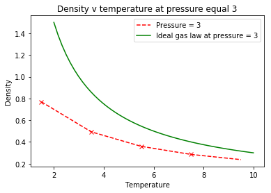
From the simulations at different densities and temperatures, comparative analysis of the density from simulation data and the data produced by the ideal gas law provided the following plots:

Figure 4 - Plot to show simulated system against ideal gas system at pressure = 3

Figure 5 - Plot to show simulated system against ideal gas system at pressure = 2

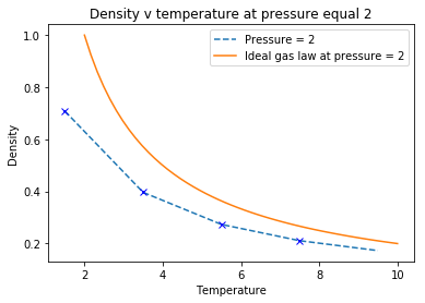The data shows that the density of the system is consistently higher than the actual system. The ideal gas law makes the assumption that the particles are volumeless points in space that have no interactions between them, unlike the Lennard-Jones which contains a repulsion term.

At low temperatures, particles possess low kinetic energy, increasing the interactions between particles. At high temperatures, the particles have increased kinetic energy, thus providing them with enough motion to reduce the density of the system through increased distances between particles to reduce unfavorable interactions, explaining the negative correlation between temperature and density. Tick

The higher pressure system ( figure 4 ) has greater discrepancy between the simulation and the ideal gas system. The increased pressure of the system means particles are more energetic so they collide more frequently resulting in increased repulsive forces causing reduced density, relative to the lower pressure ( figure 5 ) which has greater density and is more similar to the ideal gas law.Tick

The $\frac{C_v}{V}$ against temperature plot was produced by calculating the variance in energy with data provided by LAMMPS. The following plots were formed:

Figure 6 - Plot to show Temperature against $C_v/V$

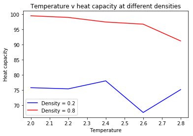For both densities, it is evident that the heat capacity does decrease as temperature increases.

The lower density system has a lower overall heat capacity. This can be rationalized via the equipartion function. The heat capacity at constant volume can be defined as

$C_v=(\frac{\partial U}{\partial T}{)}_V=\frac{3}{2}{k}_{B}N$

Where N is the number of particles in the system. Heat capacity is proportional to degrees of freedom. Both systems in this simulation contain equal volumes with different densities. Therefore it is expected that the higher density system will have a higher heat capacity because the number of particles is higher at equal volume, thus having higher degrees of freedom. Nice that you were thinking about it but I think this argument is less degrees of freedom and more density of states

The overall decrease in Heat capacity with increasing temperature can be rationalized using the Boltzmann distribution of energy states. The Boltzmann distribution is given as:

$\frac{N_i}{N}=\frac{\exp \frac{-{ϵ}_i}{KT}}{\sum _i\exp \frac{-{ϵ}_i}{KT}}$

This formula shows that that at low temperatures, the amount of higher energy states that are occupied are lower, providing vacant levels for excitation from lower energy levels at a given temperature corresponding to a high heat capacity. As the temperature increases, the occupation of higher energy states increases, deeming it more difficult for further excitation from a lower state. Therefore at higher temperatures the heat capacity is lower.Tick

The mild oscillation in the plots between 2.4 and 2.6 temperatures (larger for the lower density state) can potentially correspond to a phase change. As this simulation is plotting the heat capacity change during a melting of the crystal, the peak may correspond to the point of the phase change. Theoretically, at a phase change, the heat capacity goes to infinity as any excess energy in the system is assimilated to drive the phase change. Therefore no energy is going to change the temperature of the system until the phase change is complete, corresponding to an infinite heat capacity.Tick

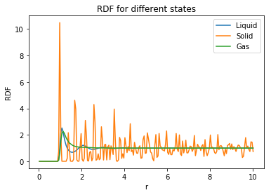
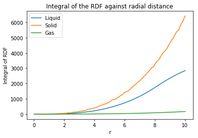
The Radial distribution function ($g(r)$) and the integral of the radial distribution function ($\int g(r)$) were plotted in order to understand the arrangement of atoms surrounding the central atom. The following plots were created:

Figure 7 - RDF of different states

Figure 8 - Integral of RDF of different states

The radial distribution function (RDF) describes the packing of the atoms within a system, thus providing a clear understanding of the atom arrangement of the system. As the internuclear distance increases (for all structures) the RDF decreases with decreased amplitude of oscillations. The RDF initially starts at zero due the typical repulsive forces that exist between the atoms in the starting arrangement at the beginning of the simulation. Not really.. ignore this. You're only interested from the peak onwards.

The gas shows a plot with one sharp peak which then immediately drops to an RDF value of 1 which corresponds to an average, evenly distributed density. Uniformity The liquid, much like the gas, starts with one sharp peak but then temporarily drops below 1 for short distances and oscillates about 1 before reaching a steady state. The liquid has a more dynamic environment than the solid, following the lennard-jones model of repulsion creating turbulent collsions at short distances. Nah, just because it's more dynamic. Particles are free to move Independence of molecules returns at large distances as the molecules separate and are free to move. However, the spacing between the peaks are not well defined, but give indication of structure at immediate distances which can be attributed to dynamic fluid shells (hydration shells in water). After the immediate shell, the probability of seeing another shell is small due to repulsion.

A solid sees a regular lattice structure with mild vibrations between fixed atoms. The plot shows an infinite number of peaks representing the spacing between the atoms in the structure. The first three peaks in the solid can be attributed to the first three layers of atoms surrounding the central atoms represented in the following image:

Figure 9 - Graphical representation of the three closest neighboring layers surrounding a central atom which correspond to the first three peaks on the RDF plot

The plot shows a steady decay of amplitude of the sharp peaks in the solid plot. The decay is due to the decrease in relative density of neighbors surrounding the center atom as r increases thus deeming it more difficult to 'find' a neighbor at a greater distance.

The liquid simulation also has a regular structure at short distances which correspond to the fluid shells. Tick but I don't like the term "fluid shells".

The integration of the RDF plot shows provides the degree of coordination of each state of matter. From analysis of the values of the plots, the solid has the highest coordination number, followed by the liquid, then the gas. This backs up the previous analysis that the solid has large coordination from surrounding atoms, due to the fixed positions of the atoms in the lattice. The smaller coordination in the liquid again can be attributed to the fluid shells surrounding atoms. The gas shows very little coordination. Tick

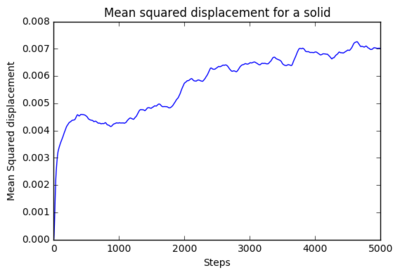
The mean squared displacement (MSD) for 8 thousand atoms and 1 million atoms were plotted. for 8 thousand atoms:

Figure 10 - MSD for vapour

Figure 11 - MSD for liquid

Figure 12 - MSD for solid

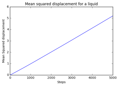
for 1 million atoms:

Figure 13 - MSD for vapour

Figure 14 - MSD for liquid

Figure 15 - MSD for solid

The gradient of the plots were calculated as the following:

	Liquid	Solid	Gas
8000 atoms	0.5034	0.2147	1.0088
1 Million atoms	0.5070	0.1804	0.9741

units?

It is evident that the from the analysis of these that the 8000 atom and the million atoms have similar results. The diffusion coefficient of the gas are both close to 1 showing rapid diffusion. The liquid diffusion coefficient is roughly about 0.5 which shows that diffusion of a liquid is less than a gas due to less freedom of the atoms within the system. The diffusion coefficient of a solid is about 0.2 which shows very little diffusion as the particles are fixed in position.What could be a benefit of a million atom simulation vs a smaller sim?

The velocity correlation function (VACF) is also a useful tool to analyse the dynamics of a liquid system as it provides the correlation between the velocity of one particle and the velocities of surrounding particles. The following plot was formed of the VACF:

Figure 16 -VACF of solid and liquid states

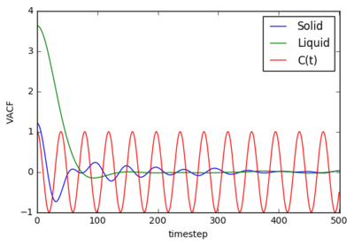The plot for the solid shows a VACF about 1 ( perfect correlations) at the instant of the simulations. Once the simulation begins, the VACF drops rapidly to below zero, thus showing negative correlation. The solid to reach it's desired structure completely outweighs the correlative property of each particle in the system. The negative term is due to immediate back-scattering after the system has reached it's desired state where the particles velocity is reversed due to collisions with a neighbor. Thus the correlation drops below zero for a moment, once the structure is reached the system will return to zero correlation after a period of oscillating about the zero point (due to further back-scattering). The Oscillations of the solid state continue for about 300 timestep, this is due to the oscillations of the particles which confined to a solid lattice. The liquid dips slightly below zero before steadying quickly to zero correlation. As time continues, the liquid particles are not locked in position and are free to move. Eventually, the particles reach distances where their velocities no longer correlate, this zero correlation.Tick, but don't get too bogged down in quantitative technicalities. The first trough represents the point at which all particles have collided exactly once, as we discussed.

The diffusion coefficient can be determined via the following equation:

	Liquid	Solid	Gas
8000 atoms	0.097888878	0.000396192	1.28436632
1 million atoms	0.090091476	4.55716E-05	1.087967925

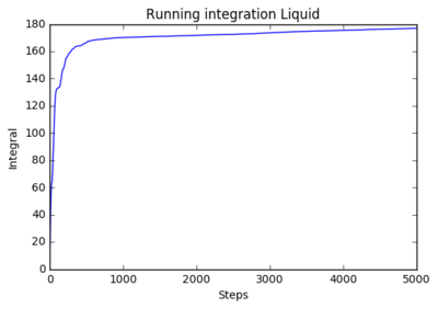
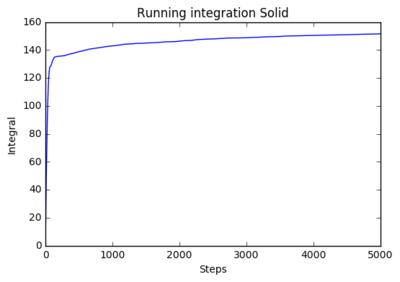
The following plots show the running integration 8000 atoms and 1 million atom systems: 8000 atoms:

Figure 17 - Running integration for gas

Figure 18 - Running integration for liquid

Figure 19- Running integration for solid

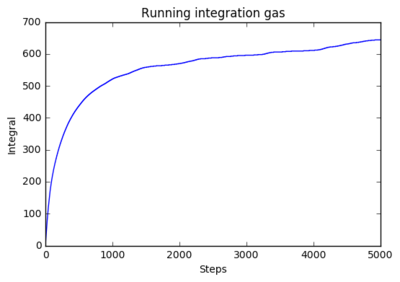
1 million atoms

Figure 20 - Running integration for gas

Figure 21 -Running integration for liquid

Figure 22 - Running integration for solid

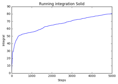The running integrals shows how the diffusion coefficient changes overtime. The solid system shows a steep initial change in diffusion coefficient as the initial system abruptly forms the natural solid structure. The plateau shows that diffusion then ceases and the system is stable. The liquid system sees a similar result where it has a steep initial movement, but not as steep as there is less ordered structure in liquids, only structure being fluid shells. The plateau for liquids is higher as diffusion continues after the initial formation of the structure. The shows a smooth curve that reaches very high values. This is expected as gasses have very little structure so move and diffuse freely.

The greatest error in the running integral is the use of the trapezium rule as this splits the area under the curve into trapeziums which neglects perfect curvature of some plots, thus potentially taking either too much or too little area under a plot.

Conclusion

Not a bad conclusion but pick and choose more the relevant stuff to include. Tie this back to the original point of the work - dynamics and phase. Have a brief philosophical moment at the end. A conclusion is always better with a "I made the world better" sentence at the end. This experiment investigated the dynamic properties of simulated matter in different states by using the LAMMPS program. The initial equilibration of the system in order to determine the tiemstep found that the most accurate timestep with the most sensible computing time was 0.0025. The comparison of the lennard-Jones potential to the Ideal Gas Law found that the density of the ideal gas system is always higher the density of the Lennard-Jones system which is attributed to the repulsive term in the Lennard-Jones equation which results in a distribution of particles in a system that tries to reduce unfavorable interactions, thus spreading out and reducing density. Both the Lennard-Jones system and the Ideal gas Law reduced in density as temperature increased from 1.5 to 9.5 (reduced units). This again can be attributed to increased kinetic energy which results in decreased density due to particles moving away from each other. The heat-capacity of two systems separated by different densities (0.2 , 0.8) found that as temperature increased from 2.0 to 2.8 (reduced units), the heat capacity decreased due to an increased occupation of higher energy levels at higher temperatures, deeming it more difficult to be excited into a higher level, thus decreasing heat capacity. The higher density (0.8) system has a higher heat capacity throughout than the lower density system (0.2) due to increased degrees of freedom in the higher density space as there are more particles per unit volume. The radial distribution functions solidified the hypothesis that solids have a regular structure, liquids have more motion and are free to move, but may contain microstructures (fluid shells) and liquids have very little ordered structure. For all experiments concerning the diffusion coefficient, it was found that the solid has extremely low diffusion coefficient (roughly 0.2), the liquid has intermediate diffusion coefficient (roughly 0.5) and gas has very high coefficient (roughly 1).

In order to improve this experiment, a wider range of densities and temperatures could be used to determine a more conclusive gradient of heat capacity against temperature. Different lattice structures could be used to see how radial distribution functions change if the arrangement of atoms are different. In order to improve the running integral analysis, a more sophisticated integration method could be used that would contain less error than the trapezium rule, i.e potentially the Simpson's rule.Tick

Tasks

Introduction to molecular dynamics simulation

Velocity Verlet Algorithm

Complete the three columns "ANALYTICAL", "ERROR", and "ENERGY": "ANALYTICAL" should contain the value of the classical solution for the position at time t, "ERROR" should contain the absolute difference between "ANALYTICAL" and the velocity-Verlet solution (i.e. ERROR should always be positive -- make sure you leave the half step rows blank!), and "ENERGY" should contain the total energy of the oscillator for the velocity-Verlet solution.

Figure 1 - Plot to show the time v energy of the 0.001 timestep plot

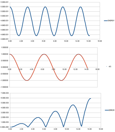For the default timestep value, 0.1, estimate the positions of the maxima in the ERROR column as a function of time. Make a plot showing these values as a function of time, and fit an appropriate function to the data.

Figure 1 - Plot to show the time v energy of the 0.001 timestep plot

Figure 1 - Plot to show the time v energy of the 0.001 timestep plot

Tick, would be nice here to put the equation of your linear fit on the graph

Experiment with different values of the timestep. What sort of a timestep do you need to use to ensure that the total energy does not change by more than 1% over the course of your "simulation"? Why do you think it is important to monitor the total energy of a physical system when modelling its behaviour numerically?

Figure 1 - Plot to show the time v energy of the 0.001 timestep plot

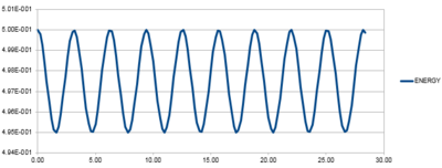By varying the timestep, the amount at which the energy varies. The above plot shows the energy oscillations at a timestep of 0.2 where the energy minimum is 4.95 (i.e. 1% of the maximum energy at 5). Any larger timestep would see an increase in error, thus showing a fluctuation of energy that is greater than 1%. Tick

It is important to monitor the total energy of a system as the fluctuations can reveal errors in the data and indicate whether the accuracy of the date is acceptable. The timestep above 0.2 sees fluctuations of 1% of the maximum energy. This can be considered a negligible amount. Any smaller timesteps may increase the accuracy of the data but the time taken to run the simulation will be increased. So the energy allows you to determine a suitable balance between accuracy and time of simulation.Tick

Lennard-Jones Potential

Find $r_0$, the seperation at which the potential energy is zero. This can be calculated from:

$\varphi (r)=4ϵ(\frac{{\sigma }^{12}}{r^{12}}-\frac{{\sigma }^6}{r^6})=0$

By rearrangement, it can be found that:

$r_0=\sigma$ When the energy is zero.Tick

The equilibrium separation $r_{eq}$ can be calculated from the differential of $\varphi$ with respect to $r$. If the differential is equated to zero it allows for the assignments of stationary points which can correspond to a minimum in energy, thus a bond.

$\frac{d\varphi }{dr}=4ϵ(\frac{-12{\sigma }^{12}}{r^{13}}+\frac{6{\sigma }^6}{r^7})=0$.

Which when rearranged provides the equilibrium distance to be $r_{eq}=2^{1/6}\sigma$.Tick

Evaluate the integrals

$\int \varphi (r)dr=\int 4ϵ(\frac{{\sigma }^{12}}{r^{12}}-\frac{{\sigma }^6}{r^6})dr$

$\underset{2\sigma }{\overset{\mathrm{\infty }}{\int }}\varphi (r)dr=-2.07x10^{-2}$

$\underset{2.5\sigma }{\overset{\mathrm{\infty }}{\int }}\varphi (r)dr=-6.81x10^{-3}$

$\underset{3\sigma }{\overset{\mathrm{\infty }}{\int }}\varphi (r)dr=-2.74x10^{-3}$Incorrect with these values, must be an accuracy thing?

Reduced Units and Masses

Estimate the number of water molecules in 1ml of water under standard conditions. Estimate the volume of 10000 water molecules under standard conditions.

As 1 ml of $H_{2}O$ is equivalent to 0.001 g.Incorrect??? 1ml = 1g Therefore the number of molecules is:

$N{o}_{H_{2}O}=\frac{0.001}{18}*6.022x10^{23}=3.55*10^{19}$ Incorrect

For the estimation of the volume of 10000 particles of $H_{2}O$ it can be assumed that:

$\frac{10000}{6.022x10^{23}}*18=Volume=2.989*10^{-19}$ Tick

Consider an atom at position $(0.5,0.5,0.5)$ in a cubic simulation box which runs from $(0,0,0)$ to $(1,1,1)$. In a single timestep, it moves along the vector $(0.7,0.6,0.2)$. At what point does it end up, after the periodic boundary conditions have been applied?.

After the motion of the vector from (0.5,0.5,0.5) along the vector (0.7,0.6,0.2), the new position $r_{new}$ is (0.2,0.1,0.7).Tick

The Lennard-Jones parameters for argon are $\sigma =0.34\mathrm{n}\mathrm{m}$, $$\begin{gathered} ϵ \\ / \\ {k}_B=120\mathrm{K} \end{gathered}$$. If the LJ cutoff is r^* = 3.2, what is it in real units? What is the well depth in $$\begin{gathered} {\mathrm{k}\mathrm{J} \\ \mathrm{m}\mathrm{o}\mathrm{l}}^{-1} \end{gathered}$$? What is the reduced temperature $T^{*}=1.5$in real units?

The real units are:

$r=3.2*0.34=1.088nm$Tick

$T=120*1.5=180K$Tick

$E=4*ϵ(\frac{0.34^{12}}{1.088^{12}}-\frac{0.34^6}{1.088^{12}})$evaluated?

Tasks required for introduction simulations

Lattice site calculations

Why do you think giving atoms random starting coordinates causes problems in simulations?

If two particles are originally positioned too close together, it can cause a repulsion which can effect the initial conditions of the system. This repulsion can lead to violent turbulence within the system, which may not be reflected of the actual system determined by the original parameters. Additionally, it is also possible, depending on the atom, two particles close enough can simulate a bond, thus reducing the density of the system. It's called blow-up :^)

Satisfy yourself that this lattice spacing corresponds to a number density of lattice points of 0.8. Consider instead a face-centred cubic lattice with a lattice point number density of 1.2. What is the side length of the cubic unit cell?

Calculation of density for simple cubic lattice

The density of the lattice points are 0.8 where: As the volume of the unit (cubic) is equal to $(length{)}^3$ where 'length' is the length of the vertices of the cubic lattice which is equal to the lattice spacing of 1.07722, then:

$Volume=1.07722^3=1.25001$.

$Density=1/volume=1/1.25001=0.8$Tick

Calculation of density for face centered lattice

As there are four lattice points per unit cell for a face centered cubic lattice, there is a different calculation for the density.

$Density=4/volume=4/(length{)}^3=1.2$

$length=\sqrt[3]{(}4/1.2)=1.494$Tick

Therefore the expected side length of a face centered cubic lattice is 1.494.

Consider again the face-centred cubic lattice from the previous task. How many atoms would be created by the create_atoms command if you had defined that lattice instead?

Considering that there is 4 atoms in the face centered cubic lattice site relative to 1 in the simple cubic system, there will be 4000 atoms created by the create_atoms command.Tick

LAMMPS Manual

Using the LAMMPS manual, find the purpose of the following commands in the input script

mass: "Set the mass for all atoms of one or more atom types. Per-type mass values can also be set in the read_data data file using the “Masses” keyword. See the units command for what mass units to use.

The I index can be specified in one of two ways. An explicit numeric value can be used, as in the 1st example above. Or a wild-card asterisk can be used to set the mass for multiple atom types. This takes the form “*” or “*n” or “n*” or “m*n”. If N = the number of atom types, then an asterisk with no numeric values means all types from 1 to N. A leading asterisk means all types from 1 to n (inclusive). A trailing asterisk means all types from n to N (inclusive). A middle asterisk means all types from m to n (inclusive)."

Pair style Command: "Set the formula(s) LAMMPS uses to compute pairwise interactions. In LAMMPS, pair potentials are defined between pairs of atoms that are within a cutoff distance and the set of active interactions typically changes over time." . "In LAMMPS, pairwise force fields encompass a variety of interactions, some of which include many-body effects, e.g. EAM, Stillinger-Weber, Tersoff, REBO potentials. They are still classified as “pairwise” potentials because the set of interacting atoms changes with time (unlike molecular bonds) and thus a neighbor list is used to find nearby interacting atoms." . The pair_style command used in this example is lj/cut 3.0 which calculate the 12/6 Lennard-Jones potential. . The Lennard-Jones potential is given as:

$E=4ϵ[(\sigma /r{)}^{12}-(\sigma /r{)}^6]$ where $r<r_c$

Where $ϵ$ is the potential well depth, $\sigma$ is the distance at which the potential between the interacting atoms is zero, r is the interparticle distance. $r_c$ is the cutoff distance.

Pair Coefficient Command "Specify the pairwise force field coefficients for one or more pairs of atom types. The number and meaning of the coefficients depends on the pair style. Pair coefficients can also be set in the data file read by the read_data command or in a restart file.

I and J can be specified in one of two ways. Explicit numeric values can be used for each, as in the 1st example above. I <= J is required. LAMMPS sets the coefficients for the symmetric J,I interaction to the same values.

A wildcard asterisk can be used in place of or in conjunction with the I,J arguments to set the coefficients for multiple pairs of atom types. This takes the form “*” or “*n” or “n*” or “m*n”. If N = the number of atom types, then an asterisk with no numeric values means all types from 1 to N. A leading asterisk means all types from 1 to n (inclusive). A trailing asterisk means all types from n to N (inclusive). A middle asterisk means all types from m to n (inclusive). Note that only type pairs with I <= J are considered; if asterisks imply type pairs where J < I, they are ignored."

Given that we are specifying ${\mathbf{x}}_i\left(0\right)$ and ${\mathbf{v}}_i\left(0\right)$, which integration algorithm are we going to use? We are going to use the Verlet Velocity algorithm as we have predetermined the parameters of the system. This will provide the atomic velocities explicitly.

The second line (starting "variable timestep...") tells LAMMPS that if it encounters the text ${timestep} on a subsequent line, it should replace it by the value given. In this case, the value ${timestep} is always replaced by 0.001. In light of this, what do you think the purpose of these lines is? Why not just write:

The ${timestep} produces a variable that allows you to manually change the timestep.

Checking Equilibration

make plots of the energy, temperature, and pressure, against time for the 0.001 timestep experiment (attach a picture to your report). Does the simulation reach equilibrium? How long does this take? When you have done this, make a single plot which shows the energy versus time for all of the timesteps (again, attach a picture to your report)

It is evident that this plot shows rapid equilibration of the liquid system, represented by the steep vertical line followed by the fluctuating horizontal plot. The blue line represents the line of best fit for the convergence section of the plot which had a gradient (calculated by polyfit function on python) of a 1.23 x 10^{-7}, which is a negligible gradient. The time required for the system to reach equilibrium was roughly 0.2 ps. Figure 3 shows the point of convergence of the 0.001 timestep energy v time plot.

The plot on figure two shows all the energy v time of each timestep calculated in the first simulation. The two lowest energy convergence are are at a timestep of 0.001 and 0.0025 (also the lowest timestep). The 0.0075 and 0.01 timestep sees increasing convergence energy respectively. The 0.015 sees no convergence and an increasing energy overall. These results can be rationalized by analysis of the simulation produced at each timestep. The 0.015 timestep would produce a simulation that sees rapid, abrupt movements, which when analysed can be interpreted by Lammps as high, potentially increasing, energy with no convergence, thus producing inaccurate results. The 0.001 and 0.0025 timesteps would produce simulations with relatively more fluid motions, where each timestep would see a convergence of the whole systems energy. The smaller timesteps also explains the smaller fluctuations of the data, due to the liquid motion. The 0.01 and 0.0075 sees increased energy the convergence due to the a slightly more abrupt motion relative to the lower energy timesteps but actually sees a convergence as the system is able to recognize the energy of the system becoming constant. Tick

Running Simulations under specific conditions

Solve the following equation for $\gamma$.

$\frac{1}{2}\sum _{n=1}^n{m}_i(v_i{)}^2=\frac{3}{2}N{k}_b\mathrm{T}$

$\frac{1}{2}\sum _{n=1}^n{m}_i(v_i{)}^2=\frac{3}{2}N{k}_b\mathrm{T}$

$\sum _{n=1}^n{m}_i(v_i{)}^2=3N{k}_b\mathrm{T}$

From the next equation:

$\frac{1}{2}\sum _{n=1}^n{m}_i(\gamma v_i{)}^2=\frac{3}{2}N{k}_B\tau$

${\gamma }^2=\frac{3N{k}_b\tau }{\sum _{n=1}^n{m}_i(v_i{)}^2}$

$\gamma =\sqrt{\frac{\tau }{T}}$ Tick

Use the manual page to find out the importance of the three numbers 100 1000 10000. How often will values of the temperature, etc., be sampled for the average? How many measurements contribute to the average? Looking to the following line, how much time will you simulate?

The general style of the fix aves function is: "fix ID group-ID ave/time Nevery Nrepeat Nfreq value1 value2 ... keyword args ..." . The 100 in this example is the Nevery which is the size of the timestep to which a value is recorded. The 1000 in this example is the Nrepeat which is the number of time to use input values for calculating averages. The 10000 is the Nfreq which is the timestep value to calculate averages.

Equations of State

When your simulations have finished, download the log files as before. At the end of the log file, LAMMPS will output the values and errors for the pressure, temperature, and density $\left(\frac{N}{V}\right)$. Use software of your choice to plot the density as a function of temperature for both of the pressures that you simulated. Your graph(s) should include error bars in both the x and y directions. You should also include a line corresponding to the density predicted by the ideal gas law at that pressure. Is your simulated density lower or higher? Justify this. Does the discrepancy increase or decrease with pressure?

These graphs show that ideally, the density of the system is consistently higher than the actual system. Be careful with wording... "the density of the ideal gas is higher than a system simulated with a Lennard-Jones forcefield" The assumptions made in the ideal gas law is that each particle does not have an individual volume and are represented as volumeless points with no interparticle interactions. Interactions between particles results in increased density as the particles are withing close proximity. At low temperatures, particles possess low kinetic energy, increasing the interactions between particles. At high temperatures, the particles have increased kinetic energy, thus providing them with enough motion to reduce the density of the system through increased distances between particles to reduce unfavorable interactions. The Lennard-Jones potential, which determines the energy required to calculate the density, contains a repulsion term, which is not included within the equation for ideal gas. The repulsion term assumes that particles in close proximity will repel each other, thus reducing the density of the system. The Ideal gas is assumed to have no repulsion, so the density is again larger. Tick

Heat Capacity

As in the last section, you need to run simulations at ten phase points. In this section, we will be in density-temperature $({\rho }^{*},T^{*})$ phase space, rather than pressure-temperature phase space. The two densities required at 0.2 and 0.8, and the temperature range is 2.0, 2.2, 2.4, 2.6, 2.8. Plot C_V/V as a function of temperature, where V is the volume of the simulation cell, for both of your densities (on the same graph). Is the trend the one you would expect? Attach an example of one of your input scripts to your report.

Figure 6 - Plot to show Temperature against $C_v/V$

For both densities, it is evident that the heat capacity does decrease as temperature increases.

The lower density system has a lower overall heat capacity. This can be rationalized via the equipartion function. The heat capacity at constant volume can be defined as

$C_v=(\frac{\partial U}{\partial T}{)}_V=\frac{3}{2}{k}_{B}N$

Where N is the number of particles in the system. Heat capacity is proportional to degrees of freedom. Both systems in this simulation contain equal volumes with different densities. Therefore it is expected that the higher density system will have a higher heat capacity because the number of particles is higher at equal volume, thus having higher degrees of freedom. Nice that you were thinking about it!

The overall decrease in Heat capacity with increasing temperature can be rationalized using the Boltzmann distribution of energy states. The Boltzmann distribution is given as:

$\frac{N_i}{N}=\frac{\exp \frac{-{ϵ}_i}{KT}}{\sum _i\exp \frac{-{ϵ}_i}{KT}}$

This formula shows that that at low temperatures, the amount of higher energy states that are occupied are lower, providing vacant levels for excitation from lower energy levels at a given temperature corresponding to a high heat capacity. As the temperature increases, the occupation of higher energy states increases, deeming it more difficult for further excitation from a lower state. Therefore at higher temperatures the heat capacity is lower.Tick

The mild oscillation in the plots between 2.4 and 2.6 temperatures (larger for the lower density state) can potentially correspond to a phase change. As this simulation is plotting the heat capacity change during a melting of the crystal, the peak may correspond to the point of the phase change. Theoretically, at a phase change, the heat capacity goes to infinity as any excess energy in the system is assimilated to drive the phase change. Therefore no energy is going to change the temperature of the system until the phase change is complete, corresponding to an infinite heat capacity.Tick

Below is a copy of my insert script

### DEFINE SIMULATION BOX GEOMETRY ###
variable dens equal 0.2
lattice sc ${dens}
region box block 0 15 0 15 0 15
create_box 1 box
create_atoms 1 box

### DEFINE PHYSICAL PROPERTIES OF ATOMS ###
mass 1 1.0
pair_style lj/cut/opt 3.0
pair_coeff 1 1 1.0 1.0
neighbor 2.0 bin

### SPECIFY THE REQUIRED THERMODYNAMIC STATE ###
variable T equal 2.0
variable timestep equal 0.0025

### ASSIGN ATOMIC VELOCITIES ###
velocity all create ${T} 12345 dist gaussian rot yes mom yes

### SPECIFY ENSEMBLE ###
timestep ${timestep}
fix nve all nve

### THERMODYNAMIC OUTPUT CONTROL ###
thermo_style custom time etotal temp press
thermo 10


### RECORD TRAJECTORY ###
dump traj all custom 1000 output-1 id x y z

### SPECIFY TIMESTEP ###

### RUN SIMULATION TO MELT CRYSTAL ###
run 10000
reset_timestep 0
unfix nve

### BRING SYSTEM TO REQUIRED STATE ###
variable tdamp equal ${timestep}*100
fix nvt all nvt temp ${T} ${T} ${tdamp}
run 10000
reset_timestep 0

### MEASURE SYSTEM STATE ###
thermo_style custom atoms step etotal temp press density
variable atoms equal atoms
variable atoms2 equal atoms*atoms
variable temp equal temp
variable temp2 equal temp*temp
variable energy equal etotal
variable energy2 equal etotal*etotal
fix aves all ave/time 100 1000 100000 v_temp v_temp2 v_energy v_energy2 v_atoms2
run 100000

variable avetemp2 equal f_aves[2]
variable aveenergy equal f_aves[3]
variable aveenergy2 equal f_aves[4]
variable aveatoms equal f_aves[5]


print "--------"

print "Tempsquared: ${avetemp2}"
print "E: ${aveenergy}"
print "E2: ${aveenergy2}"
print "Atoms: ${aveatoms}"

Radial Distribution

Perform simulations of the Lennard-Jones system in the three phases. When each is complete, download the trajectory and calculate $g(r)$ and $\int g(r)\mathrm{d}r$. Plot the RDFs for the three systems on the same axes, and attach a copy to your report. Discuss qualitatively the differences between the three RDFs, and what this tells you about the structure of the system in each phase. In the solid case, illustrate which lattice sites the first three peaks correspond to. What is the lattice spacing? What is the coordination number for each of the first three peaks?

Figure 7 - RDF of different states

Figure 8 - Integral of RDF of different states

The radial distribution function (RDF) describes the packing of the atoms within a system, thus providing a clear understanding of the atom arrangement of the system. As the internuclear distance increases (for all structures) the RDF decreases with decreased amplitude of oscillations. The RDF initially starts at zero due the typical repulsive forces that exist between the atoms in the starting arrangement at the beginning of the simulation. again not quite.. see above

The gas shows a plot with one sharp peak which then immediately drops to an RDF value of 1 which corresponds to an average, evenly distributed density. The liquid, much like the gas, starts with one sharp peak but then temporarily drops below 1 for short distances and oscillates about 1 before reaching a steady state. The liquid has a more dynamic environment than the solid, following the lennard-jones model of repulsion creating turbulent collsions at short distances. Independence of molecules returns at large distances as the molecules separate and are free to move. However, the spacing between the peaks are not well defined, but give indication of structure at immediate distances which can be attributed to dynamic fluid shells (hydration shells in water). After the immediate shell, the probability of seeing another shell is small due to repulsion.

A solid sees a regular lattice structure with mild vibrations between fixed atoms. The plot shows an infinite number of peaks representing the spacing between the atoms in the structure. The first three peaks in the solid can be attributed to the first three layers of atoms surrounding the central atoms represented in the following image:

Figure 9 - Graphical representation of the three closest neighboring layers surrounding a central atom which correspond to the first three peaks on the RDF plot

The plot shows a steady decay of amplitude of the sharp peaks in the solid plot. The decay is due to the decrease in relative density of neighbors surrounding the center atom as r increases thus deeming it more difficult to 'find' a neighbor at a greater distance.

The liquid simulation also has a regular structure at short distances which correspond to the fluid shells.

The integration of the RDF plot shows provides the degree of coordination of each state of matter. From analysis of the values of the plots, the solid has the highest coordination number, followed by the liquid, then the gas. This backs up the previous analysis that the solid has large coordination from surrounding atoms, due to the fixed positions of the atoms in the lattice. The smaller coordination in the liquid again can be attributed to the fluid shells surrounding atoms. The gas shows very little coordination.Tick, but what were your coordination numbers?

Mean Displacement Squared

make a plot for each of your simulations (solid, liquid, and gas), showing the mean squared displacement (the "total" MSD) as a function of timestep. Are these as you would expect? Estimate D in each case. Be careful with the units! Repeat this procedure for the MSD data that you were given from the one million atom simulations. The mean squared displacement for 8 thousand atoms and 1 million atoms were plotted. for 8 thousand atoms:

Figure 10 - MSD for vapour

Figure 11 - MSD for liquid

Figure 12 - MSD for solid

for 1 million atoms:

Figure 13 - MSD for vapour

Figure 14 - MSD for liquid

Figure 15 - MSD for solid

The gradient of the plots were calculated as the following:

	Liquid	Solid	Gas
8000 atoms	0.5034	0.2147	1.0088
1 Million atoms	0.5070	0.1804	0.9741

It is evident that the from the analysis of these that the 8000 atom and the million atoms have similar results. The diffusion coefficient of the gas are both close to 1 showing rapid diffusion. The liquid diffusion coefficient is roughly about 0.5 which shows that diffusion of a liquid is less than a gas due to less freedom of the atoms within the system. The diffusion coefficient of a solid is about 0.2 which shows very little diffusion as the particles are fixed in position.

Velocity Autocorrelation Function

Below is the simplification of the autocorrelation function.

$\frac{\underset{-\mathrm{\infty }}{\overset{\mathrm{\infty }}{\int }}{A}^2{\omega }^2\sin (\omega t+\varphi )\sin (\omega t+\omega \tau +\varphi )dt}{\underset{-\mathrm{\infty }}{\overset{\mathrm{\infty }}{\int }}{A}^2{\omega }^2{\sin }^2(\omega t+\varphi )dt}=\frac{\underset{-\mathrm{\infty }}{\overset{\mathrm{\infty }}{\int }}\frac{1}{2}[\cos (-\omega t)-\cos (2\omega t+\omega \tau +2\varphi )]dt}{\underset{-\mathrm{\infty }}{\overset{\mathrm{\infty }}{\int }}\frac{1}{2}[1-\cos (2\omega t+2\varphi )dt}$

$=[\frac{t\cos (-\omega \tau )-\frac{1}{2\omega }\sin (2\omega t+\omega \tau +2\varphi )}{t-\frac{1}{2\omega }\sin (2\omega t+2\varphi )}{]}_{-\mathrm{\infty }}^{\mathrm{\infty }}$

$=[\frac{\cos (-\omega \tau )-\frac{1}{2\omega t}\sin (2\omega t+\omega \tau +2\varphi )}{1-\frac{1}{2\omega t}\sin (2\omega t+2\varphi )}{]}_{-\mathrm{\infty }}^{\mathrm{\infty }}$

$\frac{cos(-\omega \tau )-0}{1-0}=cos(\omega \tau )$

VACF Plot

Figure 16 -VACF of solid and liquid states

The plot for the solid shows a VACF about 1 ( perfect correlations) at the instant of the simulations. Once the simulation begins, the VACF drops rapidly to below zero, thus showing negative correlation. The solid to reach it's desired structure completely outweighs the correlative property of each particle in the system. The negative term is due to immediate back-scattering after the system has reached it's desired state where the particles velocity is reversed due to collisions with a neighbor. Thus the correlation drops below zero for a moment, once the structure is reached the system will return to zero correlation after a period of oscillating about the zero point (due to further back-scattering). The Oscillations of the solid state continue for about 300 timestep, this is due to the oscillations of the particles which confined to a solid lattice. The liquid dips slightly below zero before steadying quickly to zero correlation. As time continues, the liquid particles are not locked in position and are free to move. Eventually, the particles reach distances where their velocities no longer correlate, this zero correlation. Tick but be sure to see the wood for the trees. Don't let quantitative technicalities shroud your understanding which should be purely and simple collision based rationalisation here

The diffusion coefficient can be determined via the following equation:

	Liquid	Solid	Gas
8000 atoms	0.097888878	0.000396192	1.28436632
1 million atoms	0.090091476	4.55716E-05	1.087967925

Units?

Running Integral

The following plots show the running integration 8000 atoms and 1 million atom systems: 8000 atoms:

Figure 17 - Running integration for gas

Figure 18 - Running integration for liquid

Figure 19- Running integration for solid

1 million atoms

Figure 20 - Running integration for gas

Figure 21 -Running integration for liquid

Figure 22 - Running integration for solid

The running integrals shows how the diffusion coefficient changes overtime. The solid system shows a steep initial change in diffusion coefficient as the initial system abruptly forms the natural solid structure. The plateau shows that diffusion then ceases and the system is stable. The liquid system sees a similar result where it has a steep initial movement, but not as steep as there is less ordered structure in liquids, only structure being fluid shells. The plateau for liquids is higher as diffusion continues after the initial formation of the structure. The shows a smooth curve that reaches very high values. This is expected as gasses have very little structure so move and diffuse freely.

The greatest error in the running integral is the use of the trapezium rule as this splits the area under the curve into trapeziums which neglects perfect curvature of some plots, thus potentially taking either too much or too little area under a plot.

References