Talk:FlorianaM

Liquid Simulations- Computational Lab-Session 3

Molecular dynamics simulation

Task 1,2 and 3: comparison of velocity-Verlet algorithm model and classical harmonic oscillator calculations

The position of an atom at time t was calculated using two methods: the velocity-Verlet algorithm method and the classical harmonic oscillator method. These were both plotted and compared as shown in the graphs below.

The error was given as the difference between the two methods.

Analytical and Energy calculations

From the graph below, it can be seen that over time the maximum error increased linearly. Since each simulation follows on from the previous, at each time step, the accuracy of the calculation decreased.

line fitted over error - error maxima increasing over time

When experimenting with different time steps, it was found that in order for the total energy to not change by more than 1% over the simulation, the time step had to be smaller than 0.3. This is due to the fact that the lower the timestep, the smallest the energy fluctuations. Energy is supposed to be constant over time, hence the importance of monitoring total energy of a physical system and when carrying out simulations. Good explanation

Task 4- Lennard-Jones interaction

Since

$\varphi \left(r\right)=4ϵ(\frac{{\sigma }^{12}}{r^{12}}-\frac{{\sigma }^6}{r^6})$

$4ϵ(\frac{{\sigma }^{12}}{r_0^{12}}-\frac{{\sigma }^6}{r_0^6})=0$

$\frac{{\sigma }^{12}}{r_0^{12}}=\frac{{\sigma }^6}{r_0^6}$

Therefore,

$r_0=\sigma$

The Force = $\frac{d(\varphi \left(r_0\right))}{d{r}_0}$

$\frac{d(\varphi \left(r_0\right))}{d{r}_0}=4\times \frac{-12ϵ{\sigma }^{12}}{r_0^{13}}+4\times \frac{7ϵ{\sigma }^6}{r_0^7}$

$F=\frac{-48ϵ{\sigma }^{12}}{{\sigma }^{13}}+\frac{28ϵ{\sigma }^6}{{\sigma }^7}$

$F=\frac{-20ϵ}{\sigma }$ Not quite, differential of r^-6 = -6.r^-7

$r_{eq}$is distance at the maximum so it is the gradient of the L-J potential:

$r_{e}q=2^{\frac{1}{6}}\sigma$

$\frac{d(\varphi \left(r_{eq}\right))}{d{r}_{eq}}=\frac{-48ϵ{\sigma }^{12}}{r_{eq}^{13}}+\frac{28ϵ{\sigma }^6}{r_{eq}^7}$

$\varphi \left(r_{eq}\right)=4ϵ(\frac{{\sigma }^{12}}{(2^{\frac{1}{6}}\sigma {)}^{12}}-\frac{{\sigma }^6}{(2^{\frac{1}{6}}\sigma {)}^6})$

$\varphi \left(r_{eq}\right)=-ϵ$ (well depth)

$\sigma =ϵ=1.0$

$\underset{2\sigma }{\overset{\mathrm{\infty }}{\int }}\varphi \left(r\right)\mathrm{d}r=\underset{2\sigma }{\overset{k}{\int }}\varphi \left(r\right)\mathrm{d}r=[4ϵ(-\frac{{\sigma }^{12}}{11r^{11}}+\frac{{\sigma }^6}{5r^5}){]}_{2\sigma }^k$

$\underset{2\sigma }{\overset{\mathrm{\infty }}{\int }}\varphi \left(r\right)\mathrm{d}r=-4(-\frac{1^{12}}{11*2^{11}{1}^{11}}+\frac{1^6}{5*2^5{1}^5})=-0.0248$

Evaluated integrals:

$\underset{2\sigma }{\overset{\mathrm{\infty }}{\int }}\varphi \left(r\right)\mathrm{d}r=-0.0248$ $\underset{2.5\sigma }{\overset{\mathrm{\infty }}{\int }}\varphi \left(r\right)\mathrm{d}r=-0.00818$ $\underset{3\sigma }{\overset{\mathrm{\infty }}{\int }}\varphi \left(r\right)\mathrm{d}r=-0.00329$ Tick

Task 5: water molecules in 1ml of water and the volume of 1000 water molecules

water molecules in 1 ml of water = 3.3455*10(^22)

volume of 1000 water molecules = 2.989*10^(-23) liters May have been nice to show the calcs

Task 6:

atom at position $(0.5,0.5,0.5)$ in a cubic simulation box which runs from $(0,0,0)$ to $(1,1,1)$. In a single timestep, it moves along the vector $(0.7,0.6,0.2)$. After the periodic boundary conditions have been applied the atom ends up at : $(0.2,0.1,0.7)$

Task 7:A

The Lennard-Jones parameters for argon are $$\begin{gathered} \sigma =0.34\mathrm{n}\mathrm{m},ϵ \\ / \\ {k}_B=120\mathrm{K} \end{gathered}$$. If the LJ cutoff is , what is it in real units? What is the well depth in $$\begin{gathered} {\mathrm{k}\mathrm{J} \\ \mathrm{m}\mathrm{o}\mathrm{l}}^{-1} \end{gathered}$$? What is the reduced temperature $T^{*}=1.5$ in real units?

$r^{*}=3.2$in real units is $r=1.088$ Units?

$T=180K$

$$\begin{gathered} ϵ \\ =0.014{kJ \\ mol}^{-1} \end{gathered}$$ Tick

Equilibration

Task 8: Giving atoms same starting coords:

This would cause a problem in simulations due to lack of similarity to classical behavior. For example, if two atoms happened to be very close together, their interaction would give an error, or a negative reading, as it would be a bad model. Think about, if the coordinates were random, atomic overlaps and the large forces associated with this. The larger the forces, the smaller the timestep

Task 9: lattice spacing corresponds to number density of lattice points.

To calculate a density, number of moles,times mass, divided by volume would give the answer.

$\rho =\frac{m}{V},$

To obtain the side length of a cubit unit cell we can just take the cube root of the number density. So, a face-centered cubic lattice with a lattice point number density of 1.2 would give a side length of 1.063 Not quite, calc error

Task 11:

The command means:

line 1 = setting the mass for the atom. In this case, 1 atom with a mass of 1.0.

line 2 = pair style will calculate the pairwise interactions. In this case interactions until the distance between neighbours exceeds 0.3 in the lennard-jones potential

line 3 = pair_coeff is the interaction between different types of atoms. Which in this case are all 0.1 between all different types of atoms. Good

 
mass 1 1.0
pair_style lj/cut 3.0
pair_coeff * * 1.0 1.0

Given that we are specifying ${\mathbf{x}}_i\left(0\right)$ and ${\mathbf{v}}_i\left(0\right)$, which integration algorithm are we going to use

Being given the starting position of atoms and their velocities, means the algorithm to use is the velocity-Verlet algorithm. Good

Task 13:

The code below was written like this in order to ensure the linking of timestep and run. Had the code been written as just two lines, each time a new code was run, the entire thing would have had to be changed manually.

### SPECIFY TIMESTEP ###
variable timestep equal 0.001
variable n_steps equal floor(100/${timestep})
variable n_steps equal floor(100/0.001)
timestep ${timestep}
timestep 0.001

### RUN SIMULATION ###
run ${n_steps}
run 100000

Task 14: plots of 0.001 timestep experiment, and plots of energy vs time for all timesteps considered:

Plot of time, energy and pressure at 0.001 timestep

Graph comparing timesteps

The simulation does reach equilibrium at around time = 0.2.

The timestep chosen following analysis was 0.0025 because it was not the smallest number of timesteps but still gave good results. Timestep 0.015 was a particularly bad choice as the data does not resolve or follow the trend, showing the timesteps are too big to guarantee usable data. Interesting use of legend on the E-t, T-t and P-t graphs!

Simulation Under Specific Conditions

Task 15: Determining $\gamma$.

$\frac{1}{2}\sum _i{m}_i{v}_i^2=\frac{3}{2}N{k}_{B}T$

$\frac{1}{2}\sum _i{m}_i{\left(\gamma v_i\right)}^2=\frac{3}{2}N{k}_B\mathfrak{𝔗}$

$\frac{1}{2}\sum _i{m}_i{v}_i^2=\frac{3}{2}N{k}_{B}T$

$$\begin{gathered} {\gamma }^2\frac{1}{2}\sum _i{m}_i{\left( \\ {v}_i\right)}^2=\frac{3}{2}N{k}_B\mathfrak{𝔗} \end{gathered}$$

${\gamma }^2\frac{3}{2}N{k}_{B}T=\frac{3}{2}N{k}_B\mathfrak{𝔗}$

$\gamma =\sqrt{\frac{\mathfrak{𝔗}}{T}}$ Tick

Task 16: Relevance of 100, 1000, 100 000

the three numbers correspond to the following:

• 100 => input a value every 100 timesteps
• 1000 => number of times imput value is used to calculate an average (ie amount of values contributing to the average)
• 100 000 => calculate averages every 100 000 steps.

Task 17: Density as a function of temperature for pressures 2.4 and 2.7

Graphs showing changes in density at pressures 2.4 and 2.7 (reduced units)

Observations:

• As temperature increases, density decreases.
• As temperature increases, difference between ideal behavior and obtained calculated values decreases
• Increasing the pressure increases the density.
• Increasing pressure increases the standard error.
• Simulated density is lower than ideal. The difference is due to firstly the fact that the ideal gas law is for a gas and the calculation carried out was for a liquid. Gasses are able to be compressed more than liquids so the difference in density as temperature increases is higher, while in a liquid the change is not as significant. Furthermore, the ideal gas law does not consider interactions between atoms, while the calculation carried out does. This means that atom repulsion, which would decreased the difference in density as temperature increases, is not taken into consideration, Tick

Heat Capacities

Task 18: Plotting $C_V/V$ as a function of temperature, where $V$ is the volume of the simulation cell, for both of your densities (on the same graph). Is the trend the one you would expect? Attach an example of one of your input scripts to your report.

Cv/V as a function of temperature

Be careful, your graph title and your graph label describe different things

The log script for one of the files can be found here

Heat capacity was found to decrease as temperature increased

In a normal crystalline solid, the trend tends to be reversed. This is because as temperature is increased, the substance has more energy to enter quantised states, thus adding degrees of freedom to the substance. This increases the internal energy and therefore increases the heat capacity. However, in the simulation run, the crystal considered did not have these degrees of freedom available, so the change in internal energy was less significant than the change in temperature. Therefore a decrease in heat capacity was observed. Interesting but in a normal crystalline solid I would expect the heat capacity to decrease. Think about how the density of states changes with temperature.

Structural properties and the radial distribution function

Task 19: Calculating $g(r)$and $\int g(r)\mathrm{d}r$- plot of the three RDFs and illustrating lattice sites.

The parameters chosen the run the experiment are as follows:

Simulation	Density	Temperature
Liquid	0.85	1.2
Solid	1.5	1.2
Gas	0.01	1.2

The graph below shows the results obtained

g(r) as a function of time for solid, liquid and gas. G(r) integral and zoomed in solid.

The RDF plots, show the probability of finding a neighbouring atom to the one in question at a specific distance from it. For all three RDF plots, all three start at zero, due to repulsion of atoms at a short distance, and remain at zero until the first peark which occurs at the value of one (which corresponds to sigma)and is where atoms are most likely to be found. The solid one shows sharp and distinct peaks, which are linked directly to the atom arrangement and correspond to the lattice point and neighbouring atoms within the lattice. Liquid also exhibits this behavior, but to a much lesser extent, as it very quickly turns into a straight line of gradient zero. Gas on the other hand, only exhibits one sharp peak before flattening out, this is due to constant random motion of gasses as well as the wide distance between in each atom in a gas.

lattice

In the solid phase, the first three peaks to the distances between atoms in the lattice. So since it is face centered cubic, they correspond to the distances between atoms. So spacing between the first atom and the atom in the centre of the lattice is 0.975 (first peak). The unit length of a lattice is 1.675 (this is the second peak). The third peak is the distance to the next neighboring atom in the chain, which is 1.875. Tick

The integrals in the graph above (second graph of the above trio) can be used to show the number of atoms of each interaction. ie how many atoms are at that specific distance away and are interacting the same way. This is done by simply reading off the running integral at a specific distance. For example, at the first peak at 0.975 for the solid, the integral is 12, therefore there are 12 atoms interacting at that point. On the next it is 55 and the third is 87.

Dynamical properties and the diffusion coefficient

Task 20: Calculating D by MSD

Graphs for solid liquid and gas showing MSD over time

D was calculated from the gradient of each plot divided by 6 and D in reduced units was obtained.

Graphs for solid, liquid and gas showing MSD over time, for a million atoms

The plots above are those of the MSD data form the one million atom simulation. D was calculated in the same way as above to give:

	D for standard atom simulation/reduced units	D for one million atom simulation/reduced units
Liquid	1.67E-4	1.67E-4
Gas	2.3E-2.	1.77E-3
Solid	6.67E-7	8.33E-9

D increases from solid to gas. This is expected due to solids having very little freedom and inclination to diffuse as they are part of a tight lattice, while gasses diffuse much more easily.

D decreases with increasing size of system. This is due to more interactions in a larger system and due to convergence of calculations in a larger system.

Task 21:

Evaluating the normalised velocity autocorrelation function for a 1D harmonic oscillator:

$C\left(\tau \right)=\frac{\underset{-\mathrm{\infty }}{\overset{\mathrm{\infty }}{\int }}v\left(t\right)v(t+\tau )\mathrm{d}t}{\underset{-\mathrm{\infty }}{\overset{\mathrm{\infty }}{\int }}{v}^2\left(t\right)\mathrm{d}t}$

velocity is related to position therefore, the classical harmonic oscillator position was subbed into the equation above

$v\left(t\right)=\frac{dx(t)}{dt}=-A\sin (\omega t+\varphi )$

$C\left(\tau \right)=A^2\times {\omega }^2\frac{\underset{-\mathrm{\infty }}{\overset{\mathrm{\infty }}{\int }}sin(t\times \omega )v(t+\tau )\times sin(\omega (t+\tau )+\varphi )\mathrm{d}t}{A^2\times {\omega }^2\underset{-\mathrm{\infty }}{\overset{\mathrm{\infty }}{\int }}si{n}^2(\omega \times t+\varphi )\mathrm{d}t}$

$C\left(\tau \right)=\frac{\underset{-\mathrm{\infty }}{\overset{\mathrm{\infty }}{\int }}sin(t\times \omega )v(t+\tau )\times sin(\omega (t+\tau )+\varphi )\mathrm{d}t}{\underset{-\mathrm{\infty }}{\overset{\mathrm{\infty }}{\int }}si{n}^2(\omega \times t+\varphi )\mathrm{d}t}$

For ease, the derivation is continued on the document below:

Derivation :)

Tick

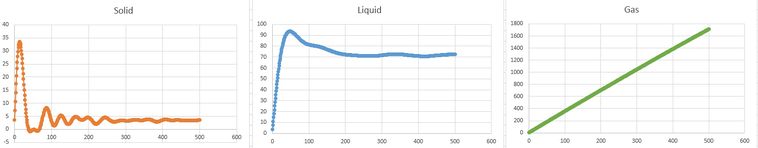
The graph below was then plotted. It is a plot of x range 0 to 500 and y range = $C\left(\tau \right)$and VACFs obtained for liquid and solid.

Graphs showing C(tau) for solid and liquid against harmonic oscillator

The harmonic oscillator is very different to liquid and solid. This is due to the impact on diffusion of collisions between molecules. Since these interactions do not feature in the harmonic oscillator (it is an approximation), the lines over time do not converge.

The liquid and solid VACFs are different due to their ability to interact and collide with molecules. Solid dips to a minimum (negative value) due to the oscillations of atoms being in the opposite direction to ζ. These oscillations then decrease and the graph flattens out due to the averaging of many atoms over time, which cancel the oscillations of each atom out. A similar trend is observed in the liquid but on a much faster scale. This is because movement of particles is much faster, therefore the trend is reached in much less time. Good

Task 22: Calculating D by VACFs

VACs calculate the velocity that a specific atom possess.

The trapezium rule was used to approximate the integral calculated above and D was estimated again.

$\underset{a}{\overset{b}{\int }}f(x)dx\approx (b-a)\left[\frac{f(a)+f(b)}{2}\right].$

calculated VACFs for solid, liquid and gas

calculated VACFs for solid, liquid and gas at 1 million atoms

D was calculated using $D=\frac{1}{3}\underset{0}{\overset{\mathrm{\infty }}{\int }}\mathrm{d}\tau ⟨\mathbf{v}\left(0\right)\cdot \mathbf{v}\left(\tau \right)⟩$.

This meant that a running integral was run and the last value was divided by 3, to calculate D.

	Standard	One Million
Solid	1.13	1.06
Liquid	24	42.4
Gas	570.6	490

The general trend is the same for both the calculated and estimated values, as expected. However there is a discrepancy in range due to general error.

The biggest source of error from the estimates could be due to particle interaction. When particles interact, they make a substantial difference to the velocity and thus effect the D value obtained. This is particularly true for gasses, hence the largest discrepancies in D values obtained. This is because in a gas, particle collisions with more force are more likely, and they will disrupt the velocity more. Would have been nice to see some more explanation on the general VACF shapes but not bad