Talk:Efr114ls

JC: General comments: Tasks which were answered were answered well with good explanations, but the questions on the RDF and VACF were missing. Make sure you attempt all of the tasks before spending too long on your answers to the earlier tasks as the later sections are more useful and more interesting.

Introduction to Molecular Dynamics Simulation

The file 'HO.xls' contains a Velocity-Verlet model for the behaviour of a classical mechanic oscillator, this file was then expanded to include:

Values for position at time $t$ using the classical mechanics model
Values for absolute difference between the classical mechanics model and the Velocity-Verlet model
Values for total energy of the system

This processed file can be accessed here: File:HOprocessedefr114.xls

Figure 2: A plot showing the relationship between maxima of absolute error against time.

The maximum deviation from the mean total energy, measured in percentage, was calculated for 20 timestep values ranging from 0.025 to 0.4. A graph and trend line were then plotted,seen in Fig.3 to produce a quadratic function and extrapolated for 1% deviation. The value of timestep used in further simulations must not exceed 0.282 - as above this value the total energy of the system fluctuations exceed the 1% limit.

The total energy of a system is one way of monitoring if the method of simulation is valid. For a simulation to be valid it must obey the 1st law of thermodynamics. Total energy is also a useful property to track the process of equilibration and can be compared with experimental data and literature to determine the accury of the simulation method.

Figure 3 A plot showing how maximum deviation from average varies with time

JC: Why does the error oscillate over time? Good, thorough analysis of the choice of timestep.

The Lennard-Jones Model

The Lennard-Jones model is widely used to describe how potential varies with distance between two non-ionic particles. It is not a completely accurate representation for a potential energy surface but its simplicity makes it an essential tool in computational chemistry.

The potential between the two particles is zero when $r_{0} = σ$ , (calculations for this can be seen below). Sigma is the equivalent of half the internuclear distance between the non bonding particles-when the particles are the same type of atom, this value is known as the Van Der Waal's radius.

The equation for the Lennard-Jones Potential for an interaction between two non ionic bodies is :

$ϕ (r) = 4 ϵ (\frac{σ^{12}}{r^{12}} - \frac{σ^{6}}{r^{6}})$

$0 = 4 ϵ (\frac{σ^{12}}{r^{12}} - \frac{σ^{6}}{r^{6}})$ $r_{0} = σ$

The force due to this interaction is given by the negative of the derivative of potential in respect to to time, resulting in:

$F (r) = - \frac{d ϕ (r)}{d r} = 24 ϵ ((\frac{σ^{6}}{r^{7}}) - 2 (\frac{σ^{12}}{r^{13}}))$

Equilibruim separation, req, is achieved when the sum of the attractive forces F(r) is equal to zero. From this equation, the equilibrium separation can be determined.

$F (r) = 0$

$\frac{σ^{6}}{r_{e q}^{7}} = 2 \frac{σ^{1} 2}{r_{e q}^{13}}$

$r_{e q}^{6} = 2 σ^{6}$

$r_{e q} = \sqrt[6]{2}$

By substituting the req value back into the Lennard-Jones potential equation, the depth of the potential and hence the energy required to fully dissociate the two atoms can be determined: phi=epsilon

$\int_{\infty}^{2 σ} ϕ (r) d r = 4 ϵ σ (\frac{1}{5} (\frac{σ^{5}}{r^{5}}) - \frac{1}{11} (\frac{σ^{11}}{r^{11}})) |_{\infty}^{2 σ} = - 2.48 * 1 0^{- 2}$

$\int_{\infty}^{2.5 σ} ϕ (r) d r = 4 ϵ σ (\frac{1}{5} (\frac{σ^{5}}{r^{5}}) - \frac{1}{11} (\frac{σ^{11}}{r^{11}})) |_{\infty}^{2.5 σ} = - 8.18 * 1 0^{- 3}$

$\int_{\infty}^{3 σ} ϕ (r) d r = 4 ϵ σ (\frac{1}{5} (\frac{σ^{5}}{r^{5}}) - \frac{1}{11} (\frac{σ^{11}}{r^{11}})) |_{\infty}^{3 σ} = = - 3.29 * 1 0^{- 3}$

JC: Correct, the force is at r = sigma so you can simplify the expression a bit more. Sigma can be thought of as the particle diameter, not the particle radius.

Periodic Boundary Conditions

Under standard conditions, the molar volume of water is $18 m L m o l^{- 1}$ , multiplication of this value by $N_{A}$ produces an estimate for the number of water molecules in a millilitre $n = 3.34 * 1 0^{22} m L^{- 1}$ . The division of this value by 10,000 gives an approximate value for the volume of 10,000 molecules of water $= 2.99 * 1 0^{- 19}$

The purpose of these calculations is to demostrate, one millimetre would corresponds to an extremely large system for calculations. Periodic Boundary conditions are essential for the simulations involved in this experiment, they allow unit cells to simulate a bulk liquid. The unit cells are projected in each direction of the axis and if an atom's trajectory leaves the unit cell, its trajectory will continue through the opposite edge of the trajectory. For example, an atom in a simple cubic unit cell that as the initial coordinates of $(0.5, 0.5, 0.5)$ and trajectory $(0.7, 0.6, 0.2)$ will have the final coordinates of $(0.7, 0.6, 0.2)$

Reduced units

Most software and literature involving Lennard-Jones potential uses reduced units. It reduces values to more managable orders of magnitude.

$r * = \frac{r}{σ}$ $E * = \frac{E}{ϵ}$ $T * = \frac{K_{B} T}{ϵ}$

Argon has the properties of $σ = 0.34 n m$ , $\frac{ϵ}{k_{B}} = 120 K$ , a Lennard-Jones cut-off value of $r * = 3.2$ and in the system $T * = 1.5$ . In real units, the Lennard jones cut-off value, $r = 1.1 n m$ and the well depth, $E_{w} = 1.0 k J m o l^{- 1}$ with a temperature of $180 K$ .

JC: All calculations correct.

Equilibration

Creating the Simulation Box

Atom postion Within the input file for a simulation, the initial positions for the atoms within the simulation box must be stated. A liquid, by definition, has no long range order so it would be a logical presumption to use randomly generated atomic coordinates, however this method can be problematic as it allows the creation of two atoms in close proximity. The issue involved with two atoms with separation of less than $σ$ is that, as seen in the Lennard-Jones plot, the potential between the atoms rapidly increases and tends to infinity. The creation of an intial state containing these high potentials and hence high energies would result in LAMMPS running to error and crashing when the simulation was run, unless an extremely small timestep is used- which limits the range of calculations possible.

JC: Good.

The set up and conditions of the simulation don’t necessarily have to correspond to exact equilibrium conditions to occur, the conditions must be in a realistic range to equilibrium conditions, allowing the use of ordered particle coordinates. A primitive cubic lattice and other basic lattice structures may be used to control initial inter-atomic distances, preventing the issues that arise with randomization of coordinates.

In following simulations, a primitive cubic lattice is uses to order the atoms, this lattice contains one lattice point per unit cell. Simple calculations for lattice constant, $a$ (in reduced units) if lattice type and number density are known.

N u m b e r D e n s i t y = \frac{N u m b e r o f l a t t i c e p o i n t s}{V o l u m e}

0.8 = \frac{1}{a^{3}}

$a = \sqrt[3]{1.25} = 1.07722$

A face centred cubic lattice, however has 4 lattice points per unit cell as seen in Figure BLAH, but the same calculation can still be used to calculate lattive constant

N u m b e r D e n s i t y = \frac{N u m b e r o f l a t t i c e p o i n t s}{V o l u m e}

1.2 = \frac{4}{a^{3}}

$a = \sqrt[3]{\frac{4}{1.2}} = 1.49380$

Number of atoms For a box with parameters defined as:

region box block 0 10 0 10 0 10
create_box 1 box

This creates a simulation box of the dimensions of 10 lattice spacing in each axis direction which corresponds to 10 unit cells in each direction and hence 1000 unit cells overall. If the lattice type used is primitive cubic with one lattice point per unit cell, 1000 lattice points and hence 1000 atoms would be created in the simulation box. If the lattice type used is face-centred cubic(FCC) with four lattice points per unit cell, 4000 lattice points and hence 4000 atoms would be created in the simulation box.

JC: Correct.

Other parameters

The command mass [type of atom] [mass of atom] is used for setting the mass for each type of atom. The first value indicates the type of atom and the second value indicates the mass of that type of the atom. In the simulations run in this simulation only one type of atom is used and hence the code mass 1 1.0 is used, however if there were more than one type of atom being used a code such as mass 1 1.0 2 1.5 would be used.

JC: Correct, for more than one type of atom I think you would have to use two separate mass commands.

The command pair_style [type of interaction] [parameter] is used for setting the type of interactions between atoms. The first value defines the type of interaction between atoms such a Lennard-Jones lj, Embedded Atom Model eam and Stillinger-Weberswand /cut shows that there is a cutoff /coul or the lack of it shows that the presence or the absence of coloumbic interactions. The second value is the cutoff parameter in reduced distance units this value must be large than σ. The command used in the simulations in this experiment is pair_style lj/cut 3.0 determines that the type of interactions are Lennard-Jones with a cutoff of 3.0 reduced distance units and with no columbic interactions or any other interactions.

JC: Here the cutoff is applied to the Lennard-Jones potential, not a Coloumbic potential, why is a cutoff used?

The command pair_coeff [type of atom][type of atom] [coefficient] [coefficient] is used to set the force field coefficients between the type of atoms. The first two values represent the atoms that are interaction and can be either numbers to represent to specify the types of atoms interaction or two asterisks to define all of the types of atoms are interacting. The last two values define the coefficients of these interactions representing $σ$ and $ϵ$ respectively. The code used in this experiment is pair_coeff * * 1.0 1.0 determining that all types of atoms are interacting equally with each other with coefficients of 1.0 resulting in symmetrical interactions.

JC: Good.

Algorithm In the simulations in this experiment, both the initial position $x_{i} (0)$ and intial velocity $v_{i} (0)$ are specified and hence the Velocity-Verlet intergration algorithm is used. The atoms are positioned in and ordered lattice - the primitive cubic lattice and the intial velocities are randomized and generated using the Maxwell-Boltzmann distribution

The plots in Figures 4,5 and 6 are plots of reduced energy, pressure and temperature against time for a 0.001 timestep and the system can be seen to equilibrate by time 0.25. After which, the values fluctuate around the mean with deviation of less that 1%.

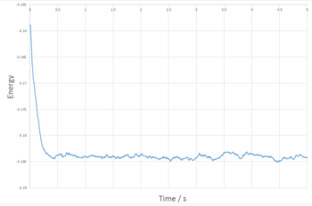
Figure 4: A plot displaying how the total energy of the system varies with time. dt=0.001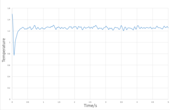
Figure 5: A plot displaying how the temperature of the system varies with time. dt=0.001
Figure 6: A plot displaying how the pressure of the system varies with time. dt=0.01

Figure 7 shows the plot of variation of total energy against time for 5 different timesteps: 0.001, 0.0025, 0.0075, 0.01 and 0.015. The timestep of 0.015 is two large and causes the total energy to diverge away from equilibrium. The remaining timesteps all converge to equilibrium successfully, however a compromise must be made between accuracy of the equilibrium total energy and length of simulation. Total energy of the system should be independant to timestep and both 0.01 and 0.0075 timesteps result in a equilibrium total energy that is significantly higher than the lower timesteps, suggesting that these timesteps are less accurate. The most suitable timestep would be 0.0025 as it has similar accuracy to 0.001 but has a longer simulation.

Figure 7: A plot that displays the relationship between total energy and time for 5 different timesteps

JC: Good choice of timestep.

Simulations Under Specific Conditions

Changes in Input File

The average kinetic energy of the system, as stated by the equipartition theorem and due to the system having three degrees of freedom (x, y, z), can be given by:

$E_{K} = \frac{1}{2} \sum_{i} m_{i} v_{i}^{2} = \frac{3}{2} N k_{B} T$

For an NpT system, the temperature must be maintained at target temperature T. In MD, the kinetic energy and hence the temperature of the system fluctuates throughout the simulation, to prevent this fluctuation from occuring, a factor of GAMMA can be introduced to correct the fluctuation which multiplies the velocity of each of the atoms by a factor to maintain a constant temperature.

$E_{K} = \frac{1}{2} \sum_{i} m_{i} (γ v_{i})^{2} = \frac{3}{2} N k_{B} 𝔗$

These two equations can then be treated simulaniously to produce the desired scaling constant- allowing the isothermal system:

$γ^{2} = \frac{𝔗}{T}$ $γ = \sqrt{\frac{𝔗}{T}}$

JC: Correct.

The input file for NpT simulations contains a command in the format of fix ID group-ID ave/time Nevery Nrepeat Nfreq value1 value2 ... keyword args ... , this determines the calculations for the thermodynamic property averages. The Nevery specifies to use input values every N timesteps,.

The Nrepeat specifies that an N number of times is used to input values to calculate averages.

The Nfreq specifies to calculate averages every N timesteps.

For this simulation, Nevery=100, Nrepeat=1000 and Nfreq=10000

In summary, 1000 input values result in the simulation of $1 * 1 0^{5}$ time units in this simulation.

JC: Make sure that you understand these three values.

The NpT Simulation

In simulations previous to this section, the ensemble being investigated was canonical (N, V, T kept constant) however in this simulation, the isothermal-isobaric ensemble is used (N, p, T kept constant). The timestep used for these simulations was 0.0025 as determined in the previous section. The pressures used were 2.5 and 3.0 in reduced units - decided due to the average temperature of 2.62 reduced unitswhen the system was in equilibrium in the previous simulations. The temperatures used were 1.60, 1.85, 2.10, 2.35 and 2.6 in reduced units - values must be greater than 1.5 as this is the critical temperature.

The ideal gas plots for pressures 2.5 and 3.0, seen in Fig.8 were calculated using the formula $ρ * = \frac{p *}{T *}$ . For both pressures tested in these simulations, the ideal gas plot results in substantially higher values for the simulation for the Lennard-Jones liquid. These differences arise from the particle modeled, both ideal gases and Lennard-Jones liquids are based on broad and contrasting assumptions. An ideal gas is composed of identical particles of negligible volume and have no intermolecular forces between particles- resulting in the total energy of the system is completely from the kinetic energy of the particles and there are no potential energy contributions. In contrast to our simulations which have Lennard-Jones interactions between particles in the system resulting in a non-zero potential. The discrepancy between the two models decreases and the temperature values increase, this could be due to the fact that at higher temperatures, average kinetic energy of the particles increases and contributes more to the total energy of the system and hence Lennard-Jones fluid behaves more alike to an ideal gas with an increase of temperature.

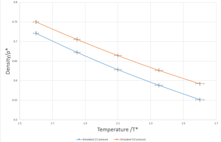
Figure 8: A figure displaying the relationship between density and temperature for an LJ fluid including error bars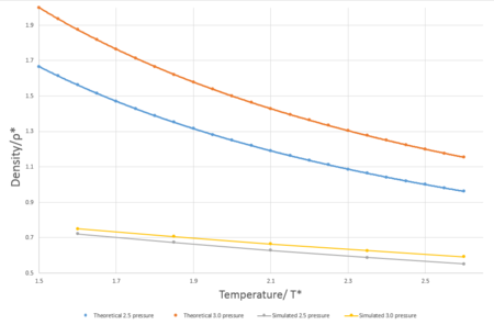
Figure 9: A figure displaying the relationship between density and temperature for both the LJ fluids and ideal gases.

JC: Specifically it is the lack of repulsive forces in the ideal gas that gives it a higher density than the Lennard-Jones simulations. The ideal gas is a good approximation to a dilute gas (high temperature and low density) as in this situation interactions between particles are less significant.

Heat Capacity Calculations

Heat capacity is the amount of energy required to heat a system by a unit temperature. It can be given using the equation:

$C_{V} = N^{2} \frac{⟨ E^{2} ⟩ - ⟨ E ⟩^{2}}{k_{B} T^{2}}$

Heat capacity per Volume can be calculated using the equation:

$C_{V} = N * ρ \frac{⟨ E^{2} ⟩ - ⟨ E ⟩^{2}}{k_{B} T^{2}}$

The $N^{2}$ variable here is a correction factor that is required due to the LAMMPS software's method of calculating heat capacity, it also provides an easy conversion of heat capacity to heat capacity per volume due to the $ρ = \frac{N}{V}$ relationship.

The ensemble used in these simulations is the canonical ensemble. In total ten simulations were run with densities of 0.8 or 0.2 in reduced units and temperatures of 2.0, 2.2, 2.4, 2.6 and 2.8 in reduced units. variable heatcap and variable heatcapperv were built into the code to calculate the heat capacity and heat capacity per volume directly. Pressure calculations were removed from the script to reduce simulation times.

$C_{V}$ was plotted as a function of temperature to produce Fig.10. Increasing the temperature of a system usually increases the specific heat capacity of a system, however as seen in Fig. 10,in this simulation and increase of the temperature of a system results in a decrease of Heat capacity for both densities. In comparison to literature, the trend is most likely due to the Frenkel line being crossed resulting in an dynamic transition from a rigid liquid to a non-rigid gas-like fluid, in this state an increase in temperature results in lower vibrational energy but higher diffusion rates which results in a reduction of internal energy. The physical definition of heat capacity $C_{V} = \frac{δ U}{δ T}$ , therefore a reduction in internal energy results in a reduction of specific heat capacity.

file://icnas4.cc.ic.ac.uk/efr114/ncomms3331.pdf

JC: Good suggestion for the trend in heat capacity with temperature, more analysis beyond the scope of this experiment would be needed to confirm this trend, why do you think heat capacity usually increases with temperature? What about the trend with density? What function did you fit to your results and why?

Below is an intro file used for the heat capacity simulations.

### DEFINE SIMULATION BOX GEOMETRY ### variable dens equal 0.8 lattice sc ${dens} region box block 0 15 0 15 0 15 create_box 1 box create_atoms 1 box ### DEFINE PHYSICAL PROPERTIES OF ATOMS ### mass 1 1.0 pair_style lj/cut/opt 3.0 pair_coeff 1 1 1.0 1.0 neighbor 2.0 bin ### SPECIFY THE REQUIRED THERMODYNAMIC STATE ### variable T equal 2.0 variable timestep equal 0.0025 ### ASSIGN ATOMIC VELOCITIES ### velocity all create ${T} 12345 dist gaussian rot yes mom yes ### SPECIFY ENSEMBLE ### timestep ${timestep} fix nve all nve ### THERMODYNAMIC OUTPUT CONTROL ### thermo_style custom time etotal temp thermo 10 ### RECORD TRAJECTORY ### dump traj all custom 1000 output-1 id x y z ### RUN SIMULATION TO MELT CRYSTAL ### run 10000 unfix nve reset_timestep 0 ### BRING SYSTEM TO REQUIRED STATE ### variable tdamp equal ${timestep}100 fix nvt all nvt temp ${T} ${T} ${tdamp} run 10000 reset_timestep 0 ### MEASURE SYSTEM STATE ### thermo_style custom step etotal temp density variable etot equal etotal variable etot2 equal etotaletotal variable temp equal temp fix aves all ave/time 100 1000 100000 v_temp v_etot v_etot2 unfix nvt fix nve all nve run 100000 variable averagetemp equal f_aves[1] variable heatcap equal (atomsatoms(f_aves[3]-f_aves[2]f_aves[2])/(f_aves[1]f_aves[1])) variable heatcapperv equal ((atoms${dens})(f_aves[3]-f_aves[2]f_aves[2])/(f_aves[1]f_aves[1])) print "Temp: ${averagetemp}" print "Heat Capacity: ${heatcap}" print "Heat Capacity per unit volume: ${heatcapperv}"

Structural Properties and the Radial Distribution Function

Phase	Temperature (reduced units)	Density (reduced units)
Vapour	1.5	0.01
Liquid	1.25	0.8
Solid	1	1.2

Dynamical Properties and the Diffusion coefficient

The MSD measures the deviation of the particles postion in respect to a standard reference position over time. Simulations for 8,000 particles were run and compared to simulations of 1,000,000 atoms. As seen below, for both 8,000 and 1,000,000 particles, the solid-state simulations have a clear trend, the MSD rapidly increases until equilibrium is reached, after which there is very minimal variation- this is because solids are not capable of undergoing brownian motion and particle motion is confined. Both the liquid-phase and the vapour-phase increase steadily with time as both fluids and vapours experience brownian motion. The system with 1,000,000 particles gives a more accurate equilibrium with less fluctuation and deviation from the main value, this is due to the large number of particles in the system, resulting in a more narrow gaussian distribution and a better defined value.

	Solid	Liquid	Vapour
8,000 particles
1,000,000 particles

Diffusion Coefficient(D)

The diffusive behaviour of the system's that were tested can be simplified into a diffusive coeffictiant, the formula for which is: $D = \frac{1}{6} \frac{δ ⟨ r^{2} (t) ⟩}{δ t}$

This can be easily determined from the linear plots to produce the values seen below.

	Diffusion Coefficient $m^{2} s^{- 1}$
	8,000 particle simulation	1,000,000 particle simulation
Vapour	1.74	3.12
Liquid	9.26*10-2	7.9810-2
Solid	-2.31*10-7	-8.75*10-7

These values are in agreement with both the MSD against time plots and with theory.

VACF's The velocity autocorrelation function can also be used to calculate the diffusion coefficient: $C (T) = ⟨ v (t) * V (t + T) ⟩$

JC: Plots look good, include the line of best fit that you used to calculate D on your plots. Why does the gas phase MSD begin as a curved line (ballistic regime)? Did you calculate D from the VACF?