Talk:Ece14 Liquid Simulation Experiment
A good attempt at the lab - most theory understood. Would have been nice to have a proper journal-like report (with a conclusion) but the dialogue you've given has been good. You write well and clearly - I would say for improvement - pick and choose what you think is important for the discussion of your ultimate aim. Here we're looking at phase behaviour so consider whether a discussion about timestep relevant to that? (just an example, which is why it might have been better to split into lab book + report to answer the tasks but to write-up the important stuff). But good: Mark 68/100
Introduction
Tick, good although the Grotthus mechanism is a very specific type of proton conduction. The dielectric constant is a measure of the polarisability so I'm not sure how these are connected Liquid simulation has become an extremely valuable area of science. Vast amounts of chemistry are performed in liquids, and understanding their behaviours enables us to better understand how to use them effectively. A particularly interesting and studied liquid is water. Unlike the simple Lennard-Jones fluids simulated in this investigation, water experiences very strong intermolecular hydrogen bonds, creating phenomena such as its high surface tension. It is notable that the length of the hydrogen bonds in water are what create its large lattice structure, making it one of the few materials to have a denser liquid phase than solid. The Grotthuss mechanism also gives water an unusually high electric constant.
The study of basic fluids such as a Lennard-Jones fluid opens the doors to research into more complex and interesting fluids and solvents, including molecular dynamics of biological fluids, making the development of methods involved in liquid simulation an exciting area of research today.
Aims and Objectives
Not a bad intro to your aims. We don't usually expand MD software abbreviations but glad you did because I didn't know what lammps stood for before :^) Also never heard of a "mathematical interaction" before..
This experiment was set up to simulate a simple Lennard-Jones fluid, and using results to analyse changes in behaviour under different conditions. The relatively large scale mathematical operations would be tedious and extremely time-consuming to even attempt by hand, so a molecular dynamics software is necessary. The software chosen for this particular investigation was the molecular dynamics simulation program Large-scale Atomic/Molecular Massively Parallel Simulator (LAMMPS). As the behaviour of fluids is dependent on the interactions of many different particles, the calculations involved in determining their mathematical interactions can become incredibly complex. This choice allows the simplification of calculations through the use of the Verlet and velocity-Verlet algorithms. These algorithms are methods of step-wise integration of complex functions, allowing approximate solutions to calculate the multiple forces acting on large numbers of particles and their resultant trajectories and behaviours.
Throughout this investigation, the software settings were optimised to provide the most accurate results with minimal computation time, and the LAMMPS software was used to control different conditions to study the change of structure and order with phase, as well as diffusion constants and heat capacities.
Theory of Computational Methods
Velocity-Verlet Integration
Accuracy of the Model
This investigation features the use of the Velocity-Verlet numerical integration algorithm as an approximate solution to calculate the changing positions and velocities of a large number of particles at once. Integration of a continuous function can prove an intensive process for many complex functions, so approximations such as this algorithm are a valuable method of reducing the computational load of simulations. The formula used involves continuous redefining of the value of when time progresses by each interval of ; these intervals are known as timesteps. In this way, a program using this algorithm does not have keep track of the velocity as it is self-starting[1], leading to lowered memory use and effectively reducing computational cost. Tick
The Velocity-Verlet algorithm is demonstrated in Fig. 1 using a simple harmonic oscillator model:

It is clear from Fig. 1 that the displacement function as calculated by the Velocity-Verlet algorithm produces a curve which aligns very closely with the continuous function. Thus the algorithm can be a very accurate approximation for a more complex function. Be more specific; here we compare the velocity-Verlet with the HO
However, as can be seen from Fig. 2, the absolute error of the Velocity-Verlet solution increases as the number of timesteps (thus the length of the simulation) increases. The self-starting nature of the algorithm, while valuable for reducing computational load, means that numerical errors are accumulated. The previous trajectory of the particle in the oscillator is not able to be "recalled" as such by the program, so only the single previous solution is assessed, and the error of each timestep calculation is added into the absolute error. Tick, good

Tick, would be nice to show the equation of the linear fit on the graph
The error in the displacement function increases as an absolute sinusoidal curve with increasing amplitude. As the harmonic oscillator and the Velocity-Verlet solutions are sinusoidal but very slightly different in period, the functions overlap increasingly poorly as the simulation continues, and the error here returns to zero every time the two functions cross. An approximate linear fit was able to illustrate the increasing maximum error; however, were the simulation able to run over a significantly longer period of time, the maxima of the error would be expected to be better represented by a sinusoidal curve. The graph's apparent deviation from zero can be readily explained by the limitations of the timestep size chosen. <span Tick
Timestep Size Optimisation
The impact of the timestep size is obvious in the calculation of the total energy of the simple harmonic oscillator. As both kinetic and potential energy terms are included, and the modelled system is isolated, it would be expected that the total energy remains constant. However, the total energies calculated from the Velocity-Verlet solutions show low level fluctuations in total energy which increase with timestep size. This error carried through from the model creates deviation from classical physical rules and must be monitored in these types of numerical approximations to avoid significant inaccuracies and poor modelling of a system's behaviour. Monitoring total energy of a system is a simple way to do this. So measuring the total energy is a way to measure the accuracy of a simulation?
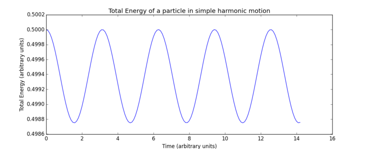
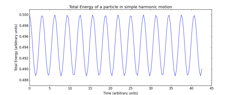
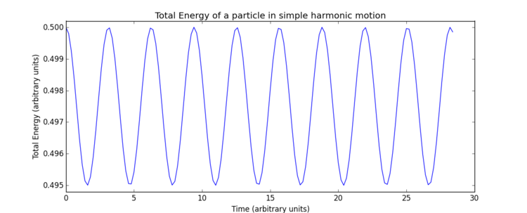
The overall error here is simply due to the nature of the model as an approximate solution. Increasing timestep () gives both a less smooth curve and an increase in oscillation amplitude, therefore, error, due to loss of information in the increasing intervals chosen. In terms of accuracy, a very small timestep is preferable, but this will require a significantly greater number of calculations to produce a simulation which runs for the same length of time - note the total time elapsed in Fig. 4 is greater than Fig. 4, ? despite identical numbers of timesteps. Consequently, when using a software such as LAMMPS, it is necessary to find a compromise through optimisation of timestep size, such that accuracy is not too significantly lost but the computational requirements remain practical. For this particular system, trial and error was able to produce an optimal timestep value of 0.200 which gives the total size of the fluctuation as of the maximum total energy value. This final error of was deemed appropriate for this experiment.Tick, good.
Atomic Forces
Due to the highly complex nature of intermolecular and interatomic forces, and the enormous computational power required to provide a solution to the Schrodinger Equation, it is necessary to use approximations to reasonably simulate the behaviour of individual molecules. This investigation uses the Lennard-Jones potential , and assumes this potential energy is the only factor inducing a force on a molecule (i.e. Coulomb force etc. are ignored). This approximation was chosen due to the relative simplicity of the function, and historical data supporting its accuracy when applied to intermolecular interactions in a simple fluid. Tick, but this is interesting. We have to think of characteristic length scales - would you use a quantum model for the dynamics of a molecular system? What is the importance of the De Broglie wavelength?
For a simple two-particle Lennard-Jones interaction:
To calculate the separation when :
Tick
It is known that the force acting on a particle due to potential energy is the negative differential of the potential energy with respect to displacement. Therefore, the force at separation may readily be calculated:
Recalling the condition :
Tick
Due to the nature of the Lennard-Jones potential only containing a single stationary point, the equilibrium separation may be easily calculated for the minimum energy position of at :
It follows that well depth is:
Tick
Specific Integrals
We may integrate the Lennard-Jones potential:
When provided with the initial conditions we can integrate within limits to obtain the following results:
Tick
Tick
Tick
These integrals show how small the area under the curve between the values of and is. Due to the extremely small area, it can be assumed that the interactions between particles at a greater separation than are negligible. Therefore, it is reasonable to set as the limit at which interactions between particles in this simulation occur, as the effect on molecular behaviours is insignificant and this saves significant computing cost.Tick, good
Periodic Boundary Conditions
The limitations of computational power mean simulations must be limited in size. A typical simulation would include between 1000 and 10000 molecules or atoms. To give a sense of scale, the number of molecules in 1g of water have been calculated for a system under standard conditions (such that density is taken to equal at ):
Tick
This is far larger a simulation than is established in this investigation. 10,000 molecules of water would take up a much smaller volume:
Tick
Tick
Tick
Thus the limitations of simulating larger scale liquids are clearly illustrated.
As a work-around to this, the simulation assumes identical repeat units surround the simulation liquid. Should a molecule in a cubic simulation box running from to begin at position and move along the vector , it would leave the box and re-enter on the opposite face to give a final position of .Tick
Units
The LAMMPS software uses reduced units for simplicity, so results of calculations on the atomic scale are given close to 1, not 1x10⁻¹⁰. Reduced units are denoted with an asterisk and are calculated using defined scaling factors.
These are demonstrated with the Lennard-Jones parameters for argon.
Given , and the Lennard-Jones cut-off as , it may be calculated in real units:
Tick
Given , and recalling well depth of the potential is :
Tick
Tick
Given the above information, temperature may also be converted to real units:
Tick
Set Up and Equilibration
Considerations in Setting Up Simulations
Unit Cells
Throughout this investigation it was decided to begin each simulation with each atom in a fixed starting point in a simple cubic lattice and allow the atoms to equilibrate from there, instead of random location generation within the simulation box. This is to prevent initial localised build-up of density, a phenomenon extremely unlikely to observe in a monatomic Lennard-Jones fluid due to increased potential energy with decreasing inter-nuclear distance. Not really, if we simulated this, the particles would just separate but nice idea Random generation would also be very likely to place atoms close together or overlapping, creating a high potential energy start point, resulting in atoms firing away from each other as though from a high energy collision - again, an unlikely observation in such a fluid. These simulations would therefore initially be poor representations of real fluids and would need to be given a much longer time to settle to equilibrium. Furthermore, the higher the potential energy of an interaction, the greater the change in velocity and position with time, so smaller timesteps would be required to accurately monitor particle behaviour. Both the increased length of simulation and decreased timestep size would increase computational cost significantly. Tick
The number density of the lattice chosen on which to set up a simulation refers to the number of lattice points per unit volume. In a simple cubic lattice with lattice point spacing of , the number density of the lattice is calculated:
Tick
Due to the lower density of the simple cubic lattice, solids will be represented using a face centred cubic lattice. With a lattice point number density of , the side length of the cubic unit cell is calculated:
Tick
When atoms in the Lennard-Jones fluid in this equilibration investigation are generated, a simulation box of 10 by 10 by 10 unit cells is generated, each containing one atom on each lattice point, totalling 1000 atoms generated. If the atoms were generated on a face centred cubic lattice instead, 4000 atoms would be generated due to the face centred cubic unit cell containing 4 identical lattice points.Tick
Examination of Input Code
As briefly mentioned previously, the Velocity-Verlet algorithm is used by LAMMPS in this investigation due to the requirements of defining both and for this simulation type. The basic Verlet algorithm is insufficient as is not defined. It is noted that while non-random initial positions are assigned, random initial velocities are able to be assigned by LAMMPS in accordance with the Maxwell Boltzmann distribution for the temperation, also defined at the beginning of the simulation.
Two sections of input code read by LAMMPS are highlighted and explained below.
mass 1 1.0
pair_style lj/cut 3.0
pair_coeff * * 1.0 1.0
This first line of code specifies that the mass of type 1 atoms in this simulation will be . Note that throughout this investigation, all simulations only use one single type of atom. The second line defines the type of interaction between atoms as a Lennard-Jones interaction, and also sets the Lennard-Jones cut-off separation as . This results in interactions between particles with separation having zero effect on each other. The third line sets the pairwise force field coefficients for all atom types (denoted by the asterisks) to be .
### SPECIFY TIMESTEP ###
variable timestep equal 0.001
variable n_steps equal floor(100/${timestep})
timestep ${timestep}

### RUN SIMULATION ###
run ${n_steps}
run 100000
This section of code is chosen to use over the much shorter:
timestep 0.001
run 100000
While they do the same thing, the first section defines timestep as a variable and calls upon it repeatedly (done using the ${timestep} notation), so it does not have to be manually adjusted at each stage in the input code. This makes the code much more manageable and makes it far easier to run multiple simulations with timestep being adjusted in each one. Tick
Running the Simulation
Initial simulations were performed where temperature, pressure and total energy of the system were monitored. These parameters are easy to measure for a real fluid, so comparisons can be drawn to experimental results to assess the accuracy of data obtained from a simulation.
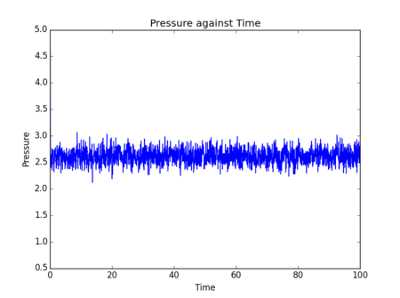
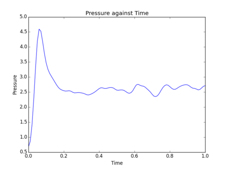
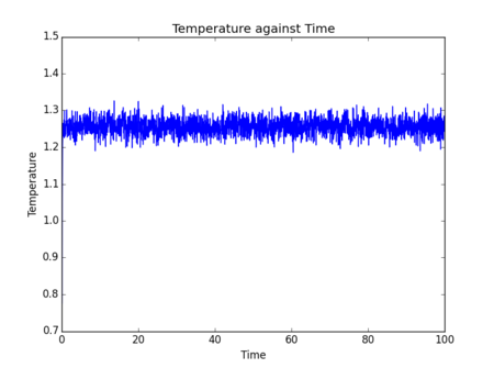
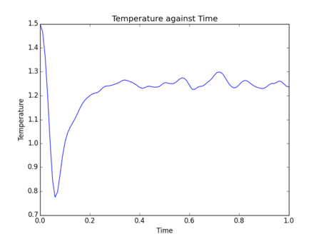
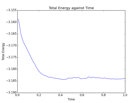
Figs. 5-10 show the results of initial simulations performed of a Lennard-Jones fluid of 1000 atoms, each initially starting on a lattice point of a 10 by 10 by 10 simple cubic lattice with other input and setup conditions chosen as described above. It can be clearly seen from all graphs that pressure, temperature and total energy all equilibrated within 0.4 clicks (time is also measured in reduced units by LAMMPS - in this instance 1 click = 48.88821 femtoseconds[2]). This rapid equilibration and resulting stable data output gives an indication that for the input parameters chosen the simulation provides an accurate representation of a Lennard-Jones fluid at equilibrium. Tick
Choosing a Timestep
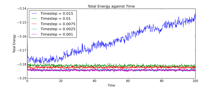
With the limitations and features of LAMMPS established as above, and the settings for the simulation adjusted accordingly, it was necessary to optimise timestep size for the liquid simulations being performed. Total energy of the same system was recorded over the period of the same simulation, with the only feature changed being the timestep size. Five timestep sizes were assessed, and the results are summarised in Fig. 11 and Table 1.
| Timestep Size | Final Total Energy Value |
|---|---|
| 0.0010 | -3.18421039 |
| 0.0025 | -3.18406602 |
| 0.0075 | -3.18224752 |
| 0.0100 | -3.18107779 |
| 0.0150 | N/A; system diverged |
It is clear that four of the five timestep sizes tested equilibrated rapidly, though to different values. The final equilibration values were calculated using an exponential decay fit and are recorded in Table 1. Through analysis of these data, it is again highlighted that the timestep size has an almost immediate effect on the ability of the system to equilibrate accurately. Due to the cumulative nature of the error, it is apparent that sufficient loss of information during the equilibration process will result in equilibration of the system, but equilibration to an inaccurate total energy value. The error cannot be rectified by extension of the length of the simulation.
The timestep 0.0150 was immediately disregarded as unsuitable for use in this type of simulation due to the significant obvious error in the results. The timestep was so large that sufficient information was lost in the initial rapid equilibration that the total energy value diverged completely, and no final value could be calculated. Comparison of the equilibrium values of total energy from timesteps 0.0075 and 0.0100 show these values too are significantly inaccurate. While the simulation still functions, the results are considered too inaccurate to use for this system. The equilibrium total energy obtained from timesteps 0.0010 and 0.0025 are, conversely, not significantly different. Therefore it can be presumed this total energy value of approximately -3.1841 is accurate. It is therefore reasonable to assume there is little advantage to the increased computational cost of a timestep of 0.0010 over the almost equally accurate 0.0025. The timestep size 0.0025 was considered most appropriate and selected for further use. Tick
Controlling Conditions
Controlling Temperature and Pressure
With a functioning simulation and appropriate timestep established, it becomes possible to control certain conditions to obtain information about the system. This experiment controls temperature, pressure and number of molecules of gas; the ensemble chosen is isothermal and isobaric.
Temperature and pressure are both controlled by constantly monitoring the temperature and pressure of the system, and updating the input information such that the output temperature and pressure are adjusted every timestep. For pressure control, the input information is updated by adjustment of the size of the simulation box. For temperature, the velocity is multiplied by a scaling factor .
For this system, refers to target temperature (that which is input into the command to control temperature), while refers to instantaneous temperature.
Using the equipartition theorem, it is possible to relate temperature to the energy of the system, and this is how a value of may be determined.
Substituting in gives:
Tick, nice
Change of Density
The change of density with respect to temperature at constant temperature and pressure was obtained by running several different liquid simulations, each at a different temperature. Average density and temperature across the simulation were reported at the end, each as an overall average. The input code for calculating this average instructed LAMMPS to take an average of each variable every 100 timesteps, and to do this 1000 times such that there were 1000 variable averages. Once 100000 timesteps had passed, these 1000 averages were to be averaged again, giving one final mean of each variable.Tick
The two pressures chosen to run these simulations of successive temperature increase were 1.8 and 2.6. These were chosen as 2.6 was approximately equivalent to the equilibrium pressure obtained from the test simulations, and 1.8 was lower than, but not far from, the fluctuations observed on the test simulation diagrams, indicating that the simulation would run with no unexpected phase changes or other behaviours.
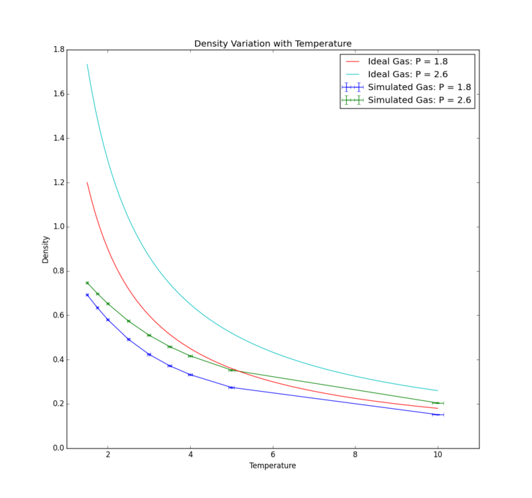
The results summarised in Fig. 12 show, for all fluids, a decrease in density as temperature is increased and pressure remains constant. This is as would be expected; an increase in temperature would lead to an increase in kinetic energy and more collisions, creating an effective pressure increase. To account for this and maintain constant pressure the volume of the system would have to increase, and this behaviour can be seen from the graph in the density decrease as . Again, as would be anticipated, the fluids held at lower pressures exhibit lower densities throughout their simulation runs due to the larger volume the fluid fills when molecules are not being forced closer together by high pressure, in accordance with the fundamental law that entropy of a system tends to a maximum.Tick
Direct comparison between the theoretical results of the ideal gas and the simulated results show that the ideal gas maintains a higher density. This is due to the ideal gas law assuming the only interaction between particles are perfect elastic collisions, whereas the simulation uses the Lennard-Jones potential, introducing repulsion between particles and decreasing density. All gases behave increasingly like perfect gases with increased temperature so this observation is expected: as atom kinetic energy increases collisions become more elastic, as the Lennard-Jones potential plays a less significant part in interactions. It is interesting that the ideal gas and simulated gas appear to converge faster at lower pressure. This can be explained by a larger intermolecular distance in lower pressure vapour leading to less Lennard-Jones interactions (recalling this simulation included an interaction cut-off of ) and more ideal gas behaviour.Tick, good. Also why does the ideal gas tend to the simulation at high T?
It is interesting to note that error in density decreases as temperature increases. This is, however, potentially a feature of the inverse proportionality between the two variables: further investigation would be required to determine if error as a percentage of the variable in question changes significantly with temperature or pressure.
Overall, it can be concluded from this data that the simulation provides a qualitatively accurate model of a fluid, and in particular a more accurate model at low temperatures than that afforded by the ideal gas law. Tick
Calculation of Heat Capacity
When performing simulations with an isobaric and isothermic ensemble, it is possible to compare results to calculate and monitor heat capacity as it changes with the ensemble variables.
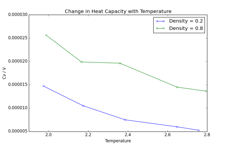
The initially obvious feature of Fig. 13 is the extremely small scale. Heat capacity in this simulation is not dependent on system volume as it is reported separately; however, as with many simple gases, the heat capacity remains very low. It is also immediately clear that the lower the density, the lower the heat capacity. This follows from the first observation: when particles are not highly spatially restricted, input energy is readily converted to kinetic energy. In a denser or more complex fluid, molecules experience more physical restrictions to motion, so kinetic energy is not increased as rapidly and more energy would be required to raise the temperature. Furthermore, Cv is heat capacity of a fixed volume. At higher pressures, there are more molecules within a given volume to heat, so naturally more energy is required. This is the opposite of what I expect and what I see. Higher density, higher heat capacity. In a denser system, more vibrations, higher density of states, higher var(E) and larger N.
A decrease in temperature resulting in decrease in heat capacity would not typically be expected, as usually the quantised internal energy levels are further apart when at high energy, so greater energy input is required to promote material to even higher energy levels. Less so this and more so defrees of freedom - translation, rotation and vibration additional terms to the Cv Indeed, as temperature becomes very high, heat capacity increases infinitely as energy levels of a material become increasingly widely spaced. However, this particular simulation runs at very low temperatures, so it is plausible that discrete vibrational energy levels are higher in density at the higher energies associated with the temperatures considered. Furthermore, it is notable that energy levels are not evenly spaced throughout the energy profile of a molecule or system, and this particular simulation is not fully representative of the wide range of conditions which may be taken into account.
An interesting feature in the higher density curve is the inconsistent downward trend. Potential reasons for this system not experiencing a decrease in heat capacity include phase changes, where energy is instead required for the latent heat of transformation. However, according to a phase diagram for a Lennard-Jones fluid[3], these conditions would result in a supercritical fluid, so phase change is unlikely. Alternatively, it could be possible that a new vibrational or rotational energy state was accessed so temperature could not be increased with as high an energy input. Further investigation would be required to understand this phenomenon.Tick
Input source code for the simulation at a density of 0.2, temperature of 2.0 and timestep = 0.0025 follows.
### DEFINE SIMULATION BOX GEOMETRY ###
variable density equal 0.2
lattice sc ${density}
region box block 0 15 0 15 0 15
create_box 1 box
create_atoms 1 box

### DEFINE PHYSICAL PROPERTIES OF ATOMS ###
mass 1 1.0
pair_style lj/cut/opt 3.0
pair_coeff 1 1 1.0 1.0
neighbor 2.0 bin

### SPECIFY THE REQUIRED THERMODYNAMIC STATE ###
variable T equal 2.0
variable timestep equal 0.0025

### ASSIGN ATOMIC VELOCITIES ###
velocity all create ${T} 12345 dist gaussian rot yes mom yes

### SPECIFY ENSEMBLE ###
timestep ${timestep}
fix nve all nve

### THERMODYNAMIC OUTPUT CONTROL ###
thermo_style custom time etotal temp press
thermo 10

### RECORD TRAJECTORY ###
dump traj all custom 1000 output-1 id x y z

### SPECIFY TIMESTEP ###

### RUN SIMULATION TO MELT CRYSTAL ###
run 10000
unfix nve
reset_timestep 0

### BRING SYSTEM TO REQUIRED STATE ###
variable tdamp equal ${timestep}*100
fix nvt all nvt temp ${T} ${T} ${tdamp}
run 10000
reset_timestep 0

unfix nvt
fix nve all nve

### MEASURE SYSTEM STATE ###
thermo_style custom step etotal temp press density
variable dens equal density
variable dens2 equal density*density
variable temp equal temp
variable temp2 equal temp*temp
variable press equal press
variable press2 equal press*press
variable atoms equal atoms
variable atoms2 equal atoms*atoms
variable energy equal etotal
variable energy2 equal etotal*etotal
fix aves all ave/time 100 1000 100000 v_dens v_temp v_press v_dens2 v_temp2 v_press2 v_energy v_energy2
run 100000

variable avedens equal f_aves[1]
variable avetemp equal f_aves[2]
variable avepress equal f_aves[3]
variable heatcap equal ${atoms2}*(f_aves[8]-(f_aves[7]*f_aves[7]))/f_aves[5]
variable errdens equal sqrt(f_aves[4]-f_aves[1]*f_aves[1])
variable errtemp equal sqrt(f_aves[5]-f_aves[2]*f_aves[2])
variable errpress equal sqrt(f_aves[6]-f_aves[3]*f_aves[3])
variable vol equal vol
variable y equal ${heatcap}/${vol}

print "Averages"
print "--------"
print "Density: ${avedens}"
print "Stderr: ${errdens}"
print "Temperature: ${avetemp}"
print "Stderr: ${errtemp}"
print "Pressure: ${avepress}"
print "Stderr: ${errpress}"
print "Heatcap: ${heatcap}"
print "CV/V: ${y}"
Different Phase Systems
Using a phase diagram for a generic Lennard-Jones fluid[4], it was possible to determine temperature and pressure combinations at which the Lennard-Jones fluid was solid, liquid or vapour. Three simulations were ran, each at a suitable temperature and pressure combination, in order to compare the Radial Distribution Functions (or RDFs, ) of the different states. The RDF is a function which describes the probability of finding another atom at a distance from any given atom in the simulation. Tick

Fig. 14 summarises the differences between radial distribution functions in different phases of Lennard-Jones materials. It is noted that there is a zero probability of finding another molecule within approximately . This is due to the repulsion between molecules at small distances being very high, so it is highly unlikely for a second atom to approach so closely, and in this simulation it appears that none do. The gas phase clearly shows a peak at what is likely , due to the stability of this particular separation resulting in instantaneous pair interactions. Beyond this, gases show no particular increased probability of finding a second atom at any distance from the first, highlighting the disordered nature of the phase. Tick The liquid phase shares this initial peak, as well as a second peak close to . This increased order could be some retention of the initial structure of the system or the formation of spheres of coordination through long-range interactions, though more likely the increased population density at these separations is due to the second closest neighbour interacting favourably with the closest neighbour. Due to the increased density of liquids, this structural order is maintained more than in the gas phase, a feature reflected in Fig. 14. Conversely, the solid phase shows comparatively extremely high order, as the probability of finding atoms at specific distances continues to very high separations. The peaks decrease in amplitude however due to vibrational motion within the solid causing long-range disorder in the simulation. It is noted that the traces for gases and liquids are far smoother than that of the liquid; this is due to the constant motion of particles leading to an even, more Gaussian, separation distribution. Solid particles are held in place by much stronger non-transient intermolecular bonds, so their motion is restricted to certain separations. Tick, good
As briefly mentioned previously, the solid simulation was not run on a simple cubic lattice, but a face centred cubic lattice. Consequently four times as many atoms were involved in the simulation. Integrals of the RDF were also calculated, and some key features were noted in that of the solid phase Lennard-Jones fluid, as seen in Fig. 15.
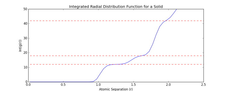
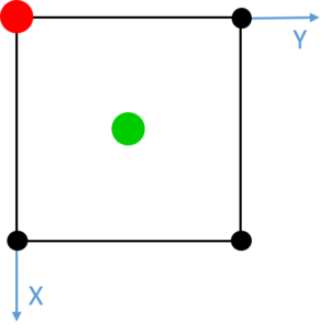
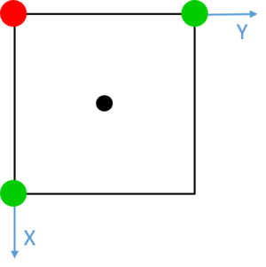
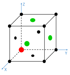
Red dashed lines have been added at each of the turning points observed between values of 0 and 2.0. The unit cell was calculated to be 1.494 in length, and these turning points match well with the distances between a given atom and its three closest neighbours. These integrals also, most notably, match extremely well with the number of neighbour atoms at each of these distances. The first turning point shows 12 neighbours at approximately , 6 neighbours at and approximately 24 neighbours at . It is noted that the turning points become increasingly unclear as the level of order of the solid decreases over distance with respect to a single atom. Similarly, due to vibrations in the structure, the precise calculated values of atomic separation are slightly lower than those observed in the simulation. However, these initial three features show clearly a trend concordant with the frequency and distance of adjacent atoms in a face centred cubic lattice. Such lattice spacings and neighbour interactions are illustrated in Figs. 16-18. Tick
Tick, v nice
Diffusion Coefficients
This final experiment explores two separate methods of calculating the diffusion coefficient associated with each of the three phases of the Lennard-Jones fluid studied. The same conditions were applied as in the RDF calculation to ensure each simulation behaved as a solid, a liquid and a gas, respectively. Data calculated by LAMMPS simulation were compared to data provided by Imperial College London for larger systems of approximately 1,000,000 atoms. For this investigation, the timestep used was reduced to 0.002 in order to match the data provided, so that simulation size is the only difference observed. Tick
Mean Squared Displacement
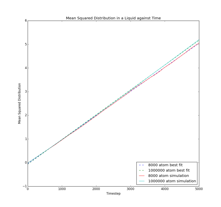
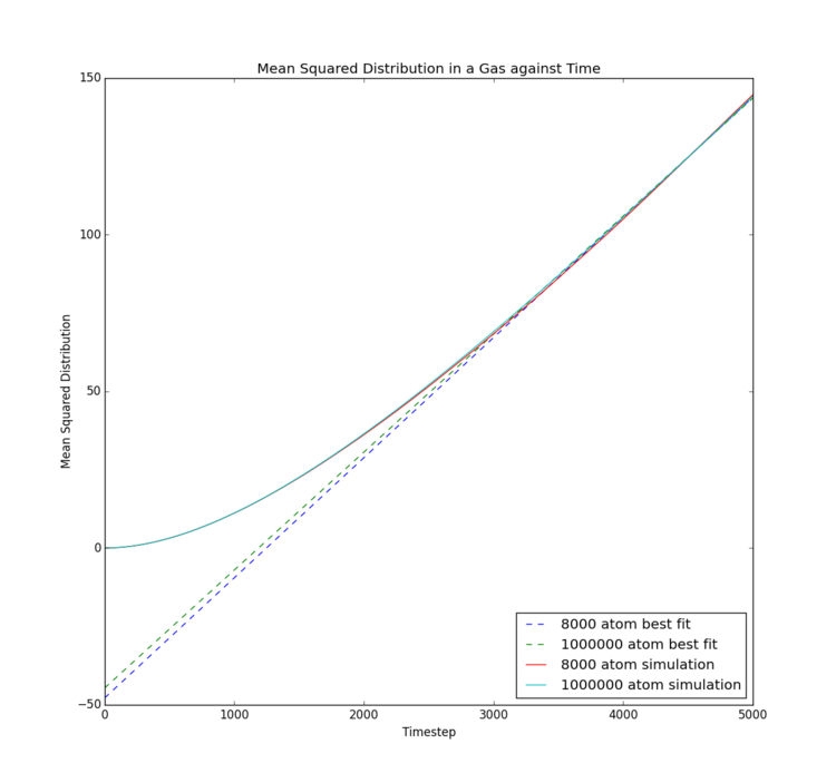
| Phase | Gradient for 8000/32000 atoms | Diffusion Coefficient for 8000/32000 atoms | Gradient for 1000000 atoms | Diffusion Coefficient for 1000000 atoms |
|---|---|---|---|---|
| Solid | 5.176 x 10⁻⁸ | 4.313 x 10⁻⁵ | -9.355 x 10⁻⁸ | -7.796 x 10⁻⁸ |
| Liquid | 0.001019 | 0.0849 | 0.001047 | 0.0873 |
| Gas | 0.03834 | 3.195 | 0.03765 | 3.138 |
Tick, units?
It is simple to calculate the diffusion coefficient from the best fit gradient of the mean squared displacement, as:
Where is the mean squared displacement.
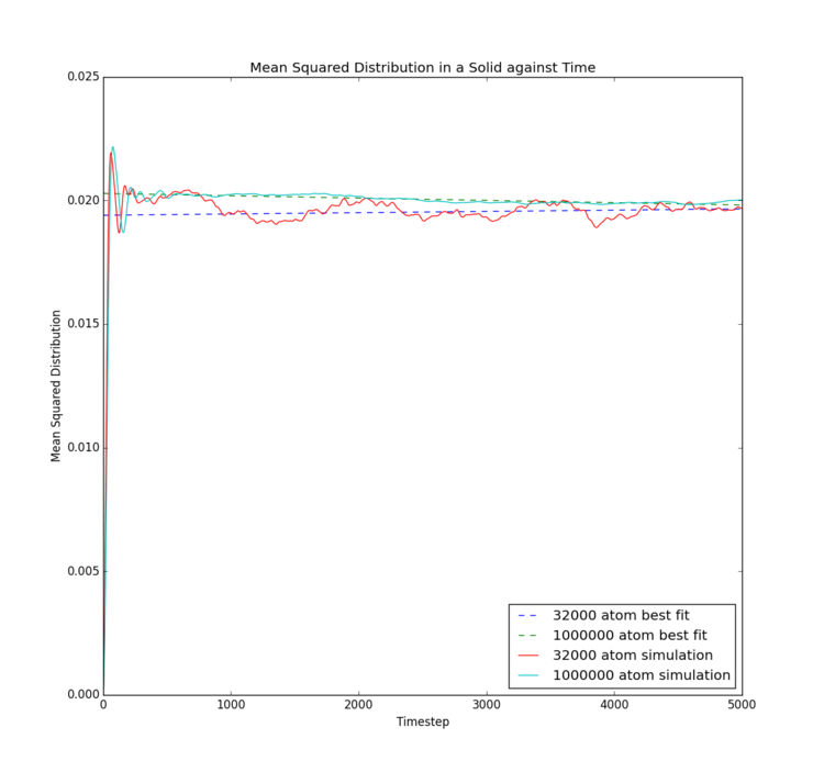
The mean squared displacement is essentially an indirect measure of the speed and extent of motion of particles in a system. For the solid phase, mean squared displacement increases suddenly, then merely fluctuates, likely with restricted vibrational motion, as the overall displacement remains relatively constant following initial equilibration. This indicates no significant displacement occurs. The liquid phase shows steady increase in displacement, indicating a single rate of motion, so that diffusion is the only method by which the liquid atoms move. The gas phase on the other hand shows intially slow displacement, which gradually increases in rate, implying diffusion is not the only force inducing motion. Potential explanations could be initial intermolecular attraction at the beginning of the simulation as atoms are released from their crystal lattice starting points; however, this would not occur in real samples and would occur to a different extent were a different timestep used. Further investigation would be necessary to obtain a better theory.
The solid provides a diffusion coefficient of very close to zero, which would be expected due to the extremely limited motion of the atoms; it can be inferred no diffusion occurs in a solid state Lennard-Jones material. As follows, the gas has the highest diffusion coefficient, indicating the gas experiences the most and fastest diffusion. Again, this makes sense, as the gas atoms experience the lowest intermolecular bonding and have greatest freedom of movement.
Interestingly, differences between the two simulation sizes are not large. It appears that with the gas phase simulation, there was essentially no difference between the two simulations, implying that the free motion of the atoms means rapid equilibration and sufficient motion to extract an accurate mean. The liquid phase also only showed a small difference in gradient of the mean squared displacement, with the smaller simulation only showing a slightly smaller mean extent of motion, potentially due to limitations of the simulation box size. The solid phase showed the most differences, as the mean squared displacement trace is significantly smoother for the larger simulation. This implies a significantly better mean could be obtained from the larger number of atoms; a common theme in statistics. The lack of impact on liquid and gas phases though implies such a large model is unnecessary.Tick
Velocity Autocorrection Function
Recalling Eq. (1):
Inputting these into :
Removal of constants and rearrangement gives:
Noting the ability to remove odd functions gives:
Giving:
Tick
This function was then plotted on the same graph as two simulated solid and gas velocity autocorrelation functions. These are useful as the integral of the velocity autocorrelation function is equivalent to the diffusion coefficient:

The harmonic oscillator in Fig. 22 shows a very clear image of a function where velocity of a particle remains dependent on its previous velocities. The function does not tend to zero. Instead, it oscillates about zero, giving a running integral of 0. This shows that a particle moving under simple harmonic motion does not diffuse at all, and its diffusion coefficient is zero.Tick
Conversely, the particles explored in the Lennard-Jones simulation do diffuse. The minima of each VACF trace indicate collisions where velocity is momentarily zero. The increased minima and maxima on the trace for a solid appear to indicate particles in a solid undergo more collisions before the velocity autocorrection function tends to zero; this is entirely plausible. For the liquid, the function appears to tend rapidly to zero, indicating sufficiently more randomised motion than in a solid that particle velocity rapidly becomes disconnected to previous velocities. The area below the curve also appears greater in the liquid simulation than in the solid, which would be concordant with previously calculated diffusion coefficient patterns. However, additional calculation would need to be performed to confirm this quantitiatively.Not quite, the minima do present collisions but not where velocity is 0
References
- ↑ 1.0 1.1 Mazur, A. K. 2008. Common Molecular Dynamics Algorithms Revisited: Accuracy and Optimal Time Steps of St¨ormer-Leapfrog Integrators. https://arxiv.org/pdf/physics/9707008.pdf - accessed 24/10/2017
- ↑ 2.0 2.1 http://lammps.sandia.gov/doc/99/units.html - accessed 24/10/2017
- ↑ 3.0 3.1 Hansen, J. & Verlet, Loup. 1969. Phase Transitions of the Lennard-Jones System. {https://link.aps.org/doi/10.1103/PhysRev.184.151} - accessed 24/10/2017
- ↑ Cite error: Invalid
<ref>tag; no text was provided for refs namedphase diagram

