Talk:Dz1814ls

JC: General comments: All tasks completed and most of the results look good. Make sure that you fully understand the background theory behind each task so that you can explain the significance of the results and how they were obtained.

Introduction to molecular dynamics

TASK 1

Complete the three columns "ANALYTICAL", "ERROR", and "ENERGY"

The given conditions were used for this simulation:

k = 1.00 | Timestep = 0.1000 | Mass = 1.00 | ɸ = 0.00 | ω = 1.00

The Analytical value was calculated using the formula above and plotted on the same graph as the result of the Velocity Verlet. As can be seen from figure 1, the values of x(t) overlap with the plot of the analytical value, showing good agreement between the classical calculation and the algorithm.

Figure 1: A position vs time plot using the classical calculation and Velocity Verlot Algorithm.

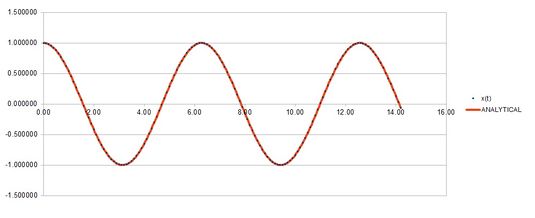
The absolute error was obtained by using the ABS() function of excel.

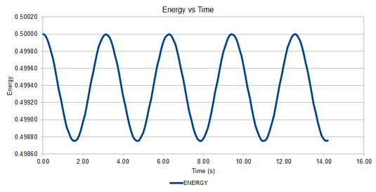
The energy was calculated using the equation above and plotted against time. The energy oscillates between 4.887 and 5.000, this is not a wide range and therefore the energy of the system can be considered to be constant.

Figure 2: A graph showing how the energy of the simulation changes over time (timestep = 0.1).

TASK 2

For the default timestep value, 0.1, estimate the positions of the maxima in the ERROR column as a function of time. Make a plot showing these values as a function of time, and fit an appropriate function to the data.

Figure 3: A graph showing the change in maximum error as a function of time.

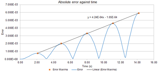
The error maxima were plotted on top of the graph of absolute error against time and were connected via a linear function of a positive gradient. As can be seen, the error of calculation increases with time. This can be explained by studying the nature of the Velocity Verlot Algorithm - since it is modeled on a Taylor expansion it is prone to an accumulation of error overtime.

JC: Why does the error oscillate?

TASK 3

Experiment with different values of the timestep. What sort of a timestep do you need to use to ensure that the total energy does not change by more than 1% over the course of your "simulation"? Why do you think it is important to monitor the total energy of a physical system when modelling its behaviour numerically?

This was done by calculating the midpoint of the energy curve - i.e the average energy - and then working out 1% of that value. The difference between the peak and trough of the energy curve was then calculated and compared to the value of 1% of the midpoint, if: energy between peak and trough > 1% of midpoint then the total energy changes more than 1% over the simulation. This was also shown graphically in the 3 figures bellow.

Figure 4: a graph of energy as a function of time at timestep = 0.1 with a 1% change limit.

Figure 5: a graph of energy as a function of time at timestep = 0.2 with a 1% change limit.

Figure 6: a graph of energy as a function of time at timestep = 0.205 with a 1% change limit.

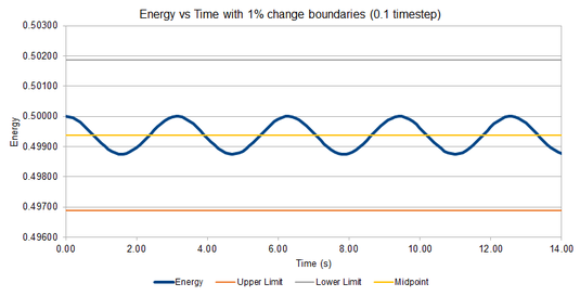
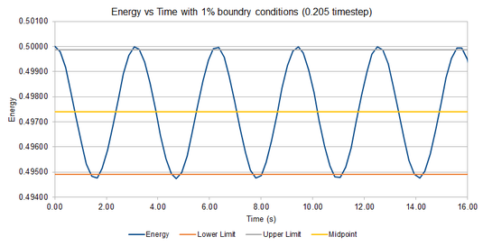
Figure 4 shows that when the chosen timestep is 0.1 the change in energy is well bellow 1% and it fluctuates quite close to the average energy of 0.499376. Increasing the timestep to 0.2 increased the fluctuation in energy, the change in energy was calculated to be 1.003%, therefore any further increase in timestep will raise the change in energy above the 1% limit. This was tested with a timestep of 0.205 (figure 6) and it can be seen that the total energy of the simulation varies by more than 1% - indicated by the curve surpassing the boundary conditions. This tells us that we must use a timestep between 0.1 and 0.2 in order to ensure the total energy of the system does not fluctuate greatly over time, this is important as in a real system obeys the law of conservation of energy and the simulation must also account for this.

JC: Good analysis and choice of timestep.

TASK 4

For a single Lennard-Jones interaction, find the separation, at which the potential energy is zero.

$\varphi \left(r\right)=4ϵ(\frac{{\sigma }^{12}}{r^{12}}-\frac{{\sigma }^6}{r^6})$

$0=4ϵ(\frac{{\sigma }^{12}}{r^{12}}-\frac{{\sigma }^6}{r^6})$

$0=\frac{{\sigma }^{12}}{r_0^{12}}-\frac{{\sigma }^6}{r_0^6}$

$0=\frac{{\sigma }^{12}}{r_0^6}-{\sigma }^6$

$r_0^6=\frac{{\sigma }^{12}}{{\sigma }^6}$

$r_0^6={\sigma }^6$

$r_0=\sigma$

What is the force at this separation?

$F=-\frac{d\varphi (r)}{dr}$

where $\varphi \left(r\right)=4ϵ(\frac{{\sigma }^{12}}{r^{12}}-\frac{{\sigma }^6}{r^6})$

$F=-\frac{d4ϵ(\frac{{\sigma }^{12}}{r^{12}}-\frac{{\sigma }^6}{r^6})}{dr}$

$F=\frac{48ϵ{\sigma }^{12}}{r_0^{13}}-\frac{24ϵ{\sigma }^6}{r_0^7}$

as shown in the previous part $r_0=\sigma$

$F=\frac{48ϵ}{\sigma }-\frac{24ϵ}{\sigma }=\frac{24ϵ}{\sigma }$

Find the equilibrium separation, and work out the well depth.

The equilibrium separation is that at which $F=0$

$F=\frac{48ϵ{\sigma }^{12}}{r_{eq}^{13}}-\frac{24ϵ{\sigma }^6}{r_{eq}^7}=0$

$\frac{48ϵ{\sigma }^{12}}{r_{eq}^{13}}=\frac{24ϵ{\sigma }^6}{r_{eq}^7}$

$48ϵ{\sigma }^{12}{r}_{eq}^7=24ϵ{\sigma }^6{r}_{eq}^{13}$

$2{\sigma }^6=r_{eq}^6$

$r_{eq}=\sqrt[6]{2}\sigma$

To calculate the well depth, $r_{eq}$ is inserted into the Lennard-Jones Equation

$\varphi \left(r\right)=4ϵ(\frac{{\sigma }^{12}}{4{\sigma }^{12}}-\frac{{\sigma }^6}{2{\sigma }^6})$

$\varphi \left(r\right)=4ϵ(\frac{1}{4}-\frac{1}{2})$

$\varphi \left(r\right)=-ϵ$

Evaluate the integrals $\underset{2\sigma }{\overset{\mathrm{\infty }}{\int }}\varphi \left(r\right)\mathrm{d}r$, $\underset{2.5\sigma }{\overset{\mathrm{\infty }}{\int }}\varphi \left(r\right)\mathrm{d}r$, and $\underset{3\sigma }{\overset{\mathrm{\infty }}{\int }}\varphi \left(r\right)\mathrm{d}r$ when $\sigma =ϵ=1.0$

$\sigma =ϵ=1$

$4\underset{x}{\overset{\mathrm{\infty }}{\int }}(\frac{1}{r^{12}}-\frac{1}{r^6})\mathrm{d}r={\left\{4(\frac{1}{5r^5}-\frac{1}{11r^{11}})\right\}}_x^{\mathrm{\infty }}=0-4(\frac{1}{5x^5}-\frac{1}{11x^{11}})$

$x=2\sigma ,\varphi \left(r\right)=-2.482*10^{-2}$

$x=2.5\sigma ,\varphi \left(r\right)=-8.176*10^{-3}$

$x=3\sigma ,\varphi \left(r\right)=-3.2901*10^{-3}$

JC: Correct.

TASK 5

Estimate the number of water molecules in 1ml of water under standard conditions. Estimate the volume of 10000 water molecules under standard conditions We know that for water 1 g = 1 mol

18.015 g (and therefore 18.015 mL) is equal to 1 mol

Therefore 1 mL = $\frac{1}{18.015}moles$

Hence the number of water molecules is equal to $\frac{1}{18.015}*N_A=3.34x10^{22}$

To estimate the volume of 10000 molecules of water, firstly calculate the amount of moles and then convert this to volume:

$\frac{10000}{N_A}=1.66*10^{-20}moles=2.99*10^{-19}c{m}^{-3}$

TASK 6

Consider an atom at position (0.5, 0.5, 0.5) in a cubic simulation box which runs from (0, 0, 0) to (1, 1, 1). In a single timestep, it moves along the vector (0.7, 0.6, 0.2). At what point does it end up, after the periodic boundary conditions have been applied?.

If the periodic boundary condition were ignored the point would end up at (1.2, 1.1, 0.7). After applying the boundary conditions, the point will end up at (0.2, 0.1, 0.7)

TASK 7

The Lennard-Jones parameters for argon are $$\begin{gathered} \sigma =0.34\mathrm{n}\mathrm{m},ϵ \\ / \\ {k}_B=120\mathrm{K} \end{gathered}$$. If the LJ cutoff is $r^{*}=3.2$, what is it in real units? What is the well depth in $$\begin{gathered} {\mathrm{k}\mathrm{J} \\ \mathrm{m}\mathrm{o}\mathrm{l}}^{-1} \end{gathered}$$? What is the reduced temperature $T^{*}=1.5$ in real units? 1. Real units of distance

$r^{*}=\frac{r}{\sigma }=3.2$

$r=3.2*3.4*10^{-8}=1.088*10^{-7}cm$

2. Real units of temperature

$T^{*}=\frac{K_{b}T}{ϵ}=1.5$

$T=1.5*120=180K$

3. Value of well depth

$ϵ=120*K_B$

$ϵ=\frac{1.6567*10^{-21}J}{1000}$

$ϵ=1.6567*10^{-24}kJ*N_A$

$ϵ=0.9977kJmo{l}^{-1}$

JC: All calculations correct and well laid out.

Equilibrium

TASK 1:

Why do you think giving atoms random starting coordinates causes problems in simulations? Hint: what happens if two atoms happen to be generated close together?

Our simulations model thousands of atoms within a single box, with a limited number of coordinates. If we were to randomly assign the starting coordinates of all these atoms, it is highly likely that some of them would either partly or fully overlap. Looking at the Lennord-Jones potential energy graph, we can see that decreasing the inter nuclear distance bellow the equilibrium length causes a sharp increase in energy and hence make the simulation significantly different to the real life conditions.

JC: The high repulsive force caused by particle overlap can make the simulation unstable and more likely to crash unless a very small timestep is used.

TASK 2:

Satisfy yourself that this lattice spacing corresponds to a number density of lattice points of 0.8. Consider instead a face-centred cubic lattice with a lattice point number density of 1.2. What is the side length of the cubic unit cell?

A cubic cell with lengths of 1.07722 will have a volume of $1.07722^3=1.25$ The number density is the number of a specified object per unit volume and is given by the following equation:

$\rho =\frac{n}{V}$

Putting the numbers in gives us $\rho =\frac{1}{1.25}=0.8$ which corresponds to the lattice point

A face-centered cubic has 4 atoms, whereas the simple cubic lattice contained one. The same equation is employed to work out the length of the sides.

$\rho =\frac{4}{V}=1.2$

$V=x^3=\frac{4}{1.2}=\frac{10}{3}$ where $x$ = length of side

$x=\sqrt[3]{\frac{10}{3}}=1.4938$

TASK 3:

Consider again the face-centred cubic lattice from the previous task. How many atoms would be created by the create_atoms command if you had defined that lattice instead?

As long as the box has the same dimensions (i.e region box block 0 10 0 10 0 10) the creat_atoms command would create 4000 atoms. This is once again due to the face-centered cubic containing 4 atoms instead of 1.

JC: Correct.

TASK 4

Using the LAMMPS manual, find the purpose of the following commands in the input script:

mass 1 1.0

This command sets up the mass for all atoms of one or more atom type. It usually takes the form of mass I value where the index I can be an explicit number or an asterisk. E.g. m*n would set all types of atoms from m to n inclusive. In the example given all atoms of type 1 have been set to a mass of 1.0.

pair_style lj/cut 3.0

This command comes in the form of pair_style style args, where style is chosen from a set list and args is the chosen variable which sets the cutoff distance of the simulation. This command is used to compute the pairwise interactions of atoms (i.e the potential) within a cutoff distance (set to 3.0 in this example). In this example the style chosen is lj/cut, this computes the Lennard-Jones potential with no Coulomb interactions given by the equation bellow, it only considers atoms within the cutoff distance of 3 (reduced units). Setting a cut off which is too small would limit the simulation and therefore produce data which is not consistent with a real life situation, whereas a large cut off limit will increase the simulation time.

$E=4ϵ\{{\left(\frac{\sigma }{r}\right)}^{12}-{\left(\frac{\sigma }{r}\right)}^6\}$ where $r<r_c$

pair_coeff * * 1.0 1.0

This command takes the form pair_coeff I J args where I and J are atom types and args are the coefficients for one or more pairs of atom types. This command sets the force field coefficients between atoms - i.e. how the atoms interact with one another, it is affected by the pair style. Once again I and J can be specified in two ways, either with an explicit number or with an asterisk - like in this example. Using an asterisk sets the coefficients for multiple pairs of atom types. In this example all the force field coefficients are set to 1.0.

JC: The force field coefficients for the Lennard-Jones potential are epsilon and sigma.

TASK 5:

Given that we are specifying ${\mathbf{x}}_i\left(0\right)$ and ${\mathbf{v}}_i\left(0\right)$, which integration algorithm are we going to use?

The Velocity-Verlot algorithm as this takes both the starting positions and their velocities.

TASK 6:

Look at the lines below.

### SPECIFY TIMESTEP ###
variable timestep equal 0.001
variable n_steps equal floor(100/${timestep})
variable n_steps equal floor(100/0.001)
timestep ${timestep}
timestep 0.001

### RUN SIMULATION ###
run ${n_steps}
run 100000

The second line (starting "variable timestep...") tells LAMMPS that if it encounters the text ${timestep} on a subsequent line, it should replace it by the value given. In this case, the value ${timestep} is always replaced by 0.001. In light of this, what do you think the purpose of these lines is? Why not just write:

timestep 0.001
run 100000

The second line sets the timestep as a variable and ensures it will always be 0.001 throughout the simulation, this is important since the number of steps is influenced by the timestep. Using the simpler code would mean that every time the timestep is changed, the number of steps would have to be changed manually. This saves time and reduces the change of making a mistake (i.e. missing out a timestep)

Task 7:

Make plots of the energy, temperature, and pressure, against time for the 0.001 timestep experiment (attach a picture to your report). Does the simulation reach equilibrium? How long does this take? When you have done this, make a single plot which shows the energy versus time for all of the timesteps (again, attach a picture to your report). Choosing a timestep is a balancing act: the shorter the timestep, the more accurately the results of your simulation will reflect the physical reality; short timesteps, however, mean that the same number of simulation steps cover a shorter amount of actual time, and this is very unhelpful if the process you want to study requires observation over a long time. Of the five timesteps that you used, which is the largest to give acceptable results? Which one of the five is a particularly bad choice? Why?

Figure 7: A graph showing the change in total energy against time at timestep t = 0.001

Figure 8: A graph showing the change of temperature against time (timestep = 0.001)

Figure 9: A graph showing the change in pressure over time at timestep t = 0.001

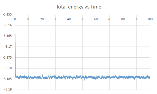
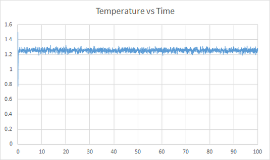
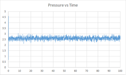
The graphs were zoomed in to the first 1 second in order to determine if the simulation had reached equilibrium. As can be seen equilibrium is reached at around t = 0.3, after this point the fluctuations of the energy, pressure and temperature remain relatively constant.

Figure 10: Total energy as a function of time (0-1 seconds)

Figure 11: Pressure as a function of time (0-1 seconds)

Figure 12: Temperature as a function of time (0-1 seconds)

Figure 13: Total energies as a function of time time for all timesteps.

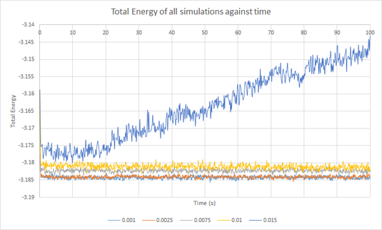
Looking at figure 13, it is clear to see that a timestep of 0.015 leads to the worst result for the total energy of the simulation and is therefore a particularly bad choice, under these condition the simulation does not reach equilibrium, possibly due to the time step being too large. At the other 4 timesteps, the system reaches equilibrium. The two timesteps of 0.001 and 0.0025 fluctuate at almost the same energy of -3.814 whilst those of 0.0075 and 0.01 fluctuate at around -3.182 and 3.181 respectively, with a larger variation around the equilibrium energy. Either timestep 0.001 or 0.0025 would work well, however the better choice would be 0.0025 as it balances accuracy with number of simulation steps.

JC: Good choice of timestep, total energy should not depend on the choice of timestep, which rules out 0.01 and 0.0075.

Running simulations under specific conditions

Task 1:

Plot the density as a function of temperature for both of the pressures that you simulated. Your graph(s) should include error bars in both the x and y directions. You should also include a line corresponding to the density predicted by the ideal gas law at that pressure. Is your simulated density lower or higher? Justify this. Does the discrepancy increase or decrease with pressure?

Figure 14: Variable section of the input file.

This part required choosing 2 pressures and 5 temperatures in order to make comparisons. In figure 11 it can be seen that the pressure average fluctuates at around P = 2.5, this was constructed using the data generated in the previous simulation (Equilibrium), hence it was chosen to use this pressure and also a slightly higher pressure of P = 3.0 for the following simulations, this was chosen as it is still relatively close to the acceptable pressure. The temperatures chosen increased by 1 up to 6.5 (including the minimum of 1.5). A timestep of 0.0025 was used as this was decided to be the best balance between accuracy and simulation steps in the previous simulation.

The data was plotted on one graph, including the predicted density (using the ideal gas law) at that pressure for comparison.

Effect of Pressure

The difference in number density between the Ideal Gas prediction and the simulated value (at T = 1.5) was calculated to be 0.924 at P = 2.5, and 1.232 at P = 3.0, showing that there is a greater discrepancy between the calculations at higher pressure. This can be explained by considering the prediction made in the ideal gas law - that particles do not interact with each other. At the lower pressure the particles in the simulation are further apart, and therefore interacting less with one another and being closer to the model of ideal gas than those at the higher pressure and therefore showing a smaller discrepancy.

Temperature

As the temperature is increased the discrepancy between the simulated value and the ideal gas prediction decreases. Once again, this is because at a higher temperature the simulation is behaving more like an ideal gas. The increased kinetic energy of the molecules can now override the inter-molecular forces which were previously acting upon them.

Figure 15: Number density as a function of temperature for simulations and as predicted by the ideal gas law at P=3 and P=2.5.

JC: Correct, the ideal gas law is a good model for a dilute gas.

Task 2:

We need to choose $\gamma$ so that the temperature is correct $T=\mathfrak{𝔗}$ if we multiply every velocity $\gamma$. We can write two equations:

$\frac{1}{2}\sum _i{m}_i{v}_i^2=\frac{3}{2}N{k}_{B}T$ $(1)$

$\frac{1}{2}\sum _i{m}_i{\left(\gamma v_i\right)}^2=\frac{3}{2}N{k}_B\mathfrak{𝔗}$ $(2)$

Solve these to determine $\gamma$.

Firstly combine equations $(1)$ + $(2)$:

$\frac{1}{2}\sum _i{m}_i{v}_i^2+\frac{1}{2}\sum _i{m}_i{\left(\gamma v_i\right)}^2=\frac{3}{2}N{k}_{B}T+\frac{3}{2}N{k}_B\mathfrak{𝔗}$

$\frac{1}{2}\sum _i{m}_i{v}_i^2+\frac{1}{2}{\gamma }^2\sum _i{m}_i{v}_i^2=\frac{3}{2}N{k}_{B}T+\frac{3}{2}N{k}_B\mathfrak{𝔗}$

$\frac{1}{2}\sum _i{m}_i{v}_i^2(1+{\gamma }^2)=\frac{3}{2}N{k}_B(T+\mathfrak{𝔗})$

Substitute in equation $(1)$:

$\frac{3}{2}N{k}_{B}T(1+{\gamma }^2)=\frac{3}{2}N{k}_B(T+\mathfrak{𝔗})$

$T(1+{\gamma }^2)=(T+\mathfrak{𝔗})$

$T+T{\gamma }^2=T+\mathfrak{𝔗}$

${\gamma }^2=\frac{\mathfrak{𝔗}}{T}$

$\gamma =\sqrt{\frac{\mathfrak{𝔗}}{T}}$

JC: Correct.

Task 3:

Use the manual page to find out the importance of the three numbers 100 1000 100000. How often will values of the temperature, etc., be sampled for the average? How many measurements contribute to the average? Looking to the following line, how much time will you simulate?

100 (nevery) - Input a value every 100 timesteps

1000 (Nrepeat)- Tells LAMMPS how many times to use the input values to calculate an average

100000 (Nfreq) - Tells LAMMPS to calculate average every 100000 timesteps

Calculating heat capacities under statistical physics

As in the last section, you need to run simulations at ten phase points. In this section, we will be in density-temperature $({\rho }^{*},T^{*})$ phase space, rather than pressure-temperature phase space. The two densities required at $0.2$ and $0.8$, and the temperature range is $2.0,2.2,2.4,2.6,2.8$. Plot $C_V/V$ as a function of temperature, where $V$ is the volume of the simulation cell, for both of your densities (on the same graph). Is the trend the one you would expect? Attach an example of one of your input scripts to your report. Bellow is the template script used to run the simulations, variable D and T were changed whilst the timestep was kept constant at 0.0025 for all simulations.

### DEFINE SIMULATION BOX GEOMETRY ###
variable D equal ...
lattice sc ${D}
region box block 0 15 0 15 0 15
create_box 1 box
create_atoms 1 box

### DEFINE PHYSICAL PROPERTIES OF ATOMS ###
mass 1 1.0
pair_style lj/cut/opt 3.0
pair_coeff 1 1 1.0 1.0
neighbor 2.0 bin

### SPECIFY THE REQUIRED THERMODYNAMIC STATE ###
variable T equal ...
variable timestep equal 0.0025

### ASSIGN ATOMIC VELOCITIES ###
velocity all create ${T} 12345 dist gaussian rot yes mom yes

### SPECIFY ENSEMBLE ###
timestep ${timestep}
fix nve all nve

### THERMODYNAMIC OUTPUT CONTROL ###
thermo_style custom time etotal temp press
thermo 10

### RECORD TRAJECTORY ###
dump traj all custom 1000 output-1 id x y z

### SPECIFY TIMESTEP ###

### RUN SIMULATION TO MELT CRYSTAL ###
run 10000
unfix nve
reset_timestep 0

### BRING SYSTEM TO REQUIRED STATE ###
variable tdamp equal ${timestep}*100
variable pdamp equal ${timestep}*1000
fix nvt all nvt temp ${T} ${T} ${tdamp} 
run 10000
reset_timestep 0

### MEASURE SYSTEM STATE ###
thermo_style custom step etotal temp atoms
variable temp equal temp
variable atoms equal atoms
variable etotal equal etotal
variable etotal2 equal etotal*etotal
fix aves all ave/time 100 1000 100000 v_temp v_etotal v_etotal2
unfix nvt
fix nve all nve
run 100000

variable temp equal f_aves[1]
variable temp2 equal temp*temp
variable etotal equal f_aves[2]
variable etotal2 equal f_aves[3]
variable atoms2 equal ${atoms}*${atoms}
variable heatcap equal ${atoms2}*(${etotal2}-${etotal}*${etotal})/${temp2}
variable volume equal vol
variable hcov equal ${heatcap}/${volume}


print "Averages"
print "--------"
print "Density: ${D}"
print "AvTemperature: ${temp}"
print "HeatCap: ${heatcap}"
print "Volume: ${volume}"
print "HeatCapOverV: ${hcov}"
print "NumAtoms: ${atoms}"

Figure 16: Heat capacity/volume as a function of temperature at Density = 0.2 and 0.8.

At a higher density, there are more atoms per unit volume. This could be seen in the simulation as the number of atoms remained constant at 3375, whilst the volume decreased from 16975 to 4218.75 as the density increased from 0.2 to 0.8. This explains the trend seen in figure 16 of an overall higher heat capacity for the higher density. The graphs also show an overall negative correlation of $\frac{C_v}{V}$ with temperature, which is counter-intuitive but can be rationalised by considering the energy bands of a crystal structure. As the temperature is increased the band gap between these energy levels decreases as they get closer and closer together and so less energy is needed for a transition between them, this could potentially result in a slightly lowered heat capacity.

JC: Good attempt at an explanation for the trend with temperature, more analysis outside the scope of this experiment would be needed to properly confirm this.

Structural properties and the radial distribution function

Perform simulations of the Lennard-Jones system in the three phases. When each is complete, download the trajectory and calculate $g(r)$ and $\int g(r)\mathrm{d}r$. Plot the RDFs for the three systems on the same axes, and attach a copy to your report. Discuss qualitatively the differences between the three RDFs, and what this tells you about the structure of the system in each phase. In the solid case, illustrate which lattice sites the first three peaks correspond to. What is the lattice spacing? What is the coordination number for each of the first three peaks?

Figure 17: RDF, g(r), as a function of distance (in reduced units) for a solid, liquid and gas phase.

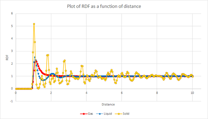
The radial distribution function, $g(r)$ describes how the density of a system varies as a function of distance - relative to a reference particle set as the origin. It can be used to give a measure of probability of finding a particle at a distance, $(r)$, away from the set origin, relative to that for an ideal gas.

As can be seen the RDF is equal to 0 for the first 0.825 reduced units of distance, placing atoms near each other at such a short distance would result in a great amount of repulsive forces and an extremely high energy. This effectively gives the width of the atoms. It is easiest to first examine and compare the RDF's for the liquid and the solid. The density of the two would differ only slightly, however a crystalline solid has long range order whilst a liquid exhibits only local order.

Liquid (Blue curve)

The peaks indicate that the atoms arrange themselves in 'shells' of nearest neighbours. The initial large peak, corresponds to the first coordination shell, and is of largest magnitude fdue to being closest to the reference atom and therefore having the strongest interactions with it. It is followed by two peaks of decreasing magnitude which could correspond to less ordered second and third coordination shells. These 3 peaks suggest that the local order extends to the first 3 neighborliness neighbors, forming the first 3 coordination shells. The RDF of the liquid eventually plateaus after a distance of 2.5 reduced units at a value of 1 which corresponds to the microscopic density of the material.

Figure 18: RDF, g(r), as a function of distance (in reduced units) for a solid, liquid and gas phase (from 0.8-2.0).

Solid (Yellow curve):

On the other hand the RDF of the solid phase shows many peaks, even at a long distance away from the reference atom - although they do decrease in magnitude - indicating a high level of order within the phase, which is expected of a crystalline solid. The first peak of the solid is noticeably sharper than that of the liquid (and the gas). This is due to the atoms within the solid being confined to a specific position within the crystalline structure, therefore they only 'move' slight distances around their lattice site unlike the atoms within a liquid which can flow around the whole system.

Gas (Red curve):

Whilst the RDF for the gaseous phase has an initial large peak, it does not correspond to there being a large number of atoms directly around the reference atom, rather it is due to the RDF being normalized to a density of unity, giving rise to the peak. The density of the gas is still extremely low and there is a large distance between the gaseous atoms.

The first 3 peaks in the RDF of the solid correspond to the 3 closest atoms which lie on different lattice coordinates of the fcc (1,2,3 in figure 18), they have the lattice spacings $(\frac{1}{2},\frac{1}{2},0),(0,1,0)(\frac{1}{2},1,\frac{1}{2})$ respectively. The second peak correspondis to the atom which is the length of a unit cell away from the reference allowing us to work out the lattice spacing simply by inspecting the second peak.

JC: Can you also calculate the lattice parameter based on the first and third peak so that you can take an average?

Figure 19: RDF, g(r), as a function of distance (in reduced units) for a solid, liquid and gas phase (from 0.8-2.0).

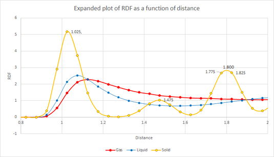
The graph was expanded between 0.8 and 2 to allow for better visualization of the first 3 solid peaks. The second peak has a value of 1.45. Therefore lattice spacing of unit cell = 1.45 reduced units. This would give a real distance of 5.075 nm using the equation from task 1.7 and the paramaters for argon $(\sigma =35nm)$.

Figure 20: Integral of g(r) over distance.

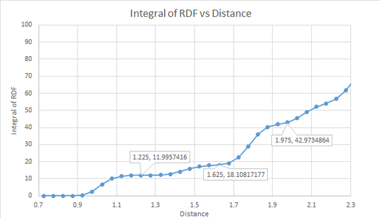
The integral of each peak corresponds to its coordination number and they were found to be 12, 6 and 18. I.E the reference atom is bound to 12 atoms at distance r=1, 6 at r=2 and 18 at r=3. This also explains the relative sizes of the peaks, there are more atoms corresponding bound to the reference which are at r=3 and hence give a larger peak than those at r=2, even though they are further away.

JC: Do these numbers of nearest neighbours make sense from the structure? There should be 24 atoms responsible for the third peak.

Dynamic properties and the diffusion coefficient

Task 1:

Make a plot for each of your simulations (solid, liquid, and gas), showing the mean squared displacement (the "total" MSD) as a function of timestep. Are these as you would expect? Estimate $D$ in each case. Be careful with the units! Repeat this procedure for the MSD data that you were given from the one million atom simulations.

To calculate the MSD of a particle you need to know its position, with respect to time - i.e. its trajectory. Plotting MSD as a function of timestep can be used to determine the situation of the particle and therefore give information about the overall system. There are 3 possible outcomes of this plot:

1) The line curves up: there is an applied force on the particle (e.g. a current flow or an applied pressure).

2) The line is straight: Only clear diffusion is acting upon the particle.

3) The line plateaus: The particle is confined.

The plots from the simulated data of 8000 atoms for gas/liquid and 32000 atoms for solid were plotted on the same graphs as the provided data for 1,000,000 atoms to allow for better comparison. It can be seen that increasing the number of atoms for each phase did not affect the shape of the graph, but simply the gradient, this therefore affected the value of the diffusion constant.

Figure 19: A plot of the Mean Squared Displacement as a function of time for the gaseous phase.

Figure 20: An expanded plot of the Mean Squared Displacement as a function of time for the gaseous phase.

Figure 21: A plot of the Mean Squared Displacement as a function of time for the liquid phase.

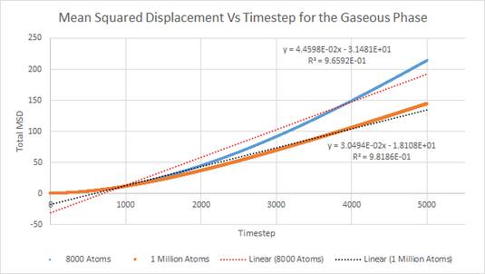
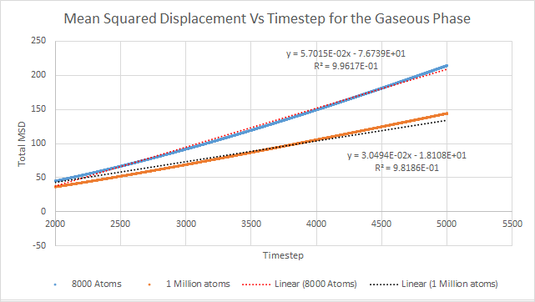
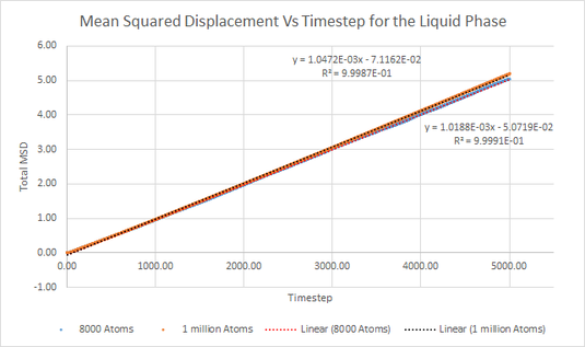
Since there is not an external force applied in the simulation, the MSD is expected to show a linear relationship for the gaseous and liquid systems simulated, however it can sometimes take some time for this to be established in the simulation as seen in figure 19 for the gaseous phase. The original MSD plot for the gaseous phase had an $R^2$ value of 0.9659, however if only the data recorded after a timestep of 2000 is considered the $R^2$ was 0.9962. By considering only this part of the data, we have allowed the system to establish the needed linear relationship. The liquid phase had a high $R^2$ value of 0.9999 without the need of any data manipulation.

JC: To get the diffusion coefficient from the MSD you should only fit to the linear part of the graph, not the entire data range. The initial curve in the gas MSD is not due to an applied force, but instead represents ballistic rather than diffusive motion.

Figure 22: A plot of the Mean Squared Displacement as a function of time for the liquid phase.

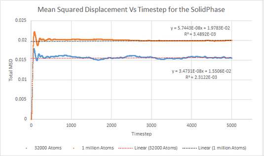
The MSD of the solid phase also follows the expected trend. It has a very short and sharp increase followed by a plateau at around an average total MSD of 0.0155, this is due to the particle in a solid being confined to a specific lattice position and not changing its position throughout the simulation. This also results in the extremely small value of MSD for the solid phase.

It can also be seen that the value of the total MSD decreases in the order Gas > Liquid > Solid, this is expected as the particle in the gaseous phase will be able to diffuse further and faster than that in a liquid as it will have less resistance from surrounding particles due to the lower density of gases. This was further confirmed by calculating the diffusion constant, the gaseous phase had the largest value whilst the solid had the smallest, which was as expected.

Calculating the Diffusion constant

The equation of $y=mx+c$ for each simulation was used to calculate the diffusion constant using the bellow equation:

$D=\frac{1}{6}\frac{\partial ⟨r^2\left(t\right)⟩}{\partial t}$ where $\frac{\partial ⟨r^2\left(t\right)⟩}{\partial t}=m$

$D=\frac{m}{6}$

The value of $m$ had to be converted into real units by dividing by the timestep.

Solid, 32,000 atoms:

$m=3.437*10^{-}8$ in reduced units

$m=1.7185*10^{-}5$ in real units

$D=2.8642*10^{-}6$

Liquid, 8,000 atoms:

$m=1.0188*10^{-}3$ in reduced units

$m=0.5094$ in real units

$D=0.0849$

Gas, 8,000 atoms

$m=5.7015*10^{-}2$ in reduced units

$m=28.5075$ in real units

$D=4.7513$

Solid, 1 Million atoms:

$m=5.7443*10^{-}8$ in reduced units

$m=2.87215*10^{-}5$ in real units

$D=4.7869*10^{-}6$

Liquid, 1 Million atoms:

$m=1.0472*10^{-}3$ in reduced units

$m=0.5236$ in real units

$D=0.0873$

Gas, 1 Million atoms:

$m=3.0494*10^{-}2$ in reduced units

$m=15.247$ in real units

$D=2.5411$

Task 2

In the theoretical section at the beginning, the equation for the evolution of the position of a 1D harmonic oscillator as a function of time was given. Using this, evaluate the normalised velocity autocorrelation function for a 1D harmonic oscillator (it is analytic!):

$C\left(\tau \right)=\frac{\underset{-\mathrm{\infty }}{\overset{\mathrm{\infty }}{\int }}v\left(t\right)v(t+\tau )\mathrm{d}t}{\underset{-\mathrm{\infty }}{\overset{\mathrm{\infty }}{\int }}{v}^2\left(t\right)\mathrm{d}t}$

The position of a 1D harmonic oscillator as a function of time is given by: $x(t)=Acos(\omega t+\varphi )$ Integrating this gives:

$v(t)=\frac{dx(t)}{dt}=-A\omega sin(\omega t+\varphi )$

Similarly when $t=t+\tau$ :

$v(t+\tau )=\frac{dx(t)}{dt}=-A\omega sin(\omega t+\omega \tau +\varphi )$

We then substitute these back into the first equation:

$C\left(\tau \right)=\frac{\underset{-\mathrm{\infty }}{\overset{\mathrm{\infty }}{\int }}-A\omega sin(\omega t+\varphi )*-A\omega sin(\omega t+\omega \tau +\varphi )\mathrm{d}t}{\underset{-\mathrm{\infty }}{\overset{\mathrm{\infty }}{\int }}(-A\omega sin(\omega t+\varphi ){)}^2\mathrm{d}t}$

$C\left(\tau \right)=\frac{A^2{\omega }^2\underset{-\mathrm{\infty }}{\overset{\mathrm{\infty }}{\int }}sin(\omega t+\varphi )*sin(\omega t+\omega \tau +\varphi )\mathrm{d}t}{A^2{\omega }^2\underset{-\mathrm{\infty }}{\overset{\mathrm{\infty }}{\int }}si{n}^2(\omega t+\varphi )\mathrm{d}t}$

$C\left(\tau \right)=\frac{\underset{-\mathrm{\infty }}{\overset{\mathrm{\infty }}{\int }}sin(\omega t+\varphi )*sin(\omega t+\omega \tau +\varphi )\mathrm{d}t}{\underset{-\mathrm{\infty }}{\overset{\mathrm{\infty }}{\int }}si{n}^2(\omega t+\varphi )\mathrm{d}t}$

Integrate the denominator:

$\underset{-\mathrm{\infty }}{\overset{\mathrm{\infty }}{\int }}si{n}^2(\omega t+\varphi )\mathrm{d}t$

$\frac{1}{2}\underset{-\mathrm{\infty }}{\overset{\mathrm{\infty }}{\int }}1-cos(2(\omega t+\varphi ))\mathrm{d}t$

$\frac{1}{2}(t-\frac{1}{2\omega }sin(2(\omega t+\varphi )))$

Integrate the numerator using:

$sin(A+B)=sin(A)cos(B)+sin(B)cos(A)$

$sin(\omega t+\omega \tau +\varphi )=sin(\omega t+\varphi )cos(\omega \tau )+sin(\omega \tau )cos(\omega t+\varphi )$

$\underset{-\mathrm{\infty }}{\overset{\mathrm{\infty }}{\int }}sin(\omega t+\varphi )sin(\omega t+\omega \tau +\varphi )=\underset{-\mathrm{\infty }}{\overset{\mathrm{\infty }}{\int }}sin(\omega t+\varphi )(sin(\omega t+\varphi )cos(\omega \tau )+sin(\omega \tau )cos(\omega t+\varphi ))$

$\underset{-\mathrm{\infty }}{\overset{\mathrm{\infty }}{\int }}si{n}^2(\omega t+\varphi )cos(\omega \tau )+sin(\omega t+\varphi )sin(\omega \tau )cos(\omega t+\varphi ))$

$\frac{cos(\tau )}{2}(t-\frac{1}{2\omega }sin(2(\omega t+\varphi )))+sin(\omega \tau )\underset{-\mathrm{\infty }}{\overset{\mathrm{\infty }}{\int }}sin(\omega t+\varphi )cos(\omega t+\varphi ))$

Using integration by substitution with $u=sin(\omega t+\varphi )$ to integrate the next part, the numerator becomes:

$\frac{cos(\omega \tau )}{2}(t-\frac{1}{2\omega }sin(2(\omega t+\varphi )))+\frac{sin(\omega \tau )}{2\omega }si{n}^2(\omega t+\varphi )$

Putting the two back together:

$C\left(\tau \right)=\frac{{\{\frac{cos(\omega \tau )}{2}(t-\frac{1}{2\omega }sin(2(\omega t+\varphi )))+\frac{sin(\omega \tau )}{2\omega }si{n}^2(\omega t+\varphi )\}}_{-\mathrm{\infty }}^{\mathrm{\infty }}}{{\left\{\frac{1}{2}(t-\frac{1}{2\omega }sin(2(\omega t+\varphi )))\right\}}_{-\mathrm{\infty }}^{\mathrm{\infty }}}$

This cancels down because of the limits being infinity, i.e Sin(t) would be so small compared to t = infinity that it can be neglected.

$C(\tau )={\left\{\frac{tcos(\omega \tau )}{2}\right\}}_{-\mathrm{\infty }}^{\mathrm{\infty }}/{\left\{\frac{t}{2}\right\}}_{-\mathrm{\infty }}^{\mathrm{\infty }}$

$C(\tau )=cos(\omega \tau )$

JC: You can calculate the answer without performing any integration by simplifying the numerator into a sin squared term and a sin x cos term which is an odd function and hence the integral is zero.

Task 3

On the same graph, with x range 0 to 500, plot $C\left(\tau \right)$ with $\omega =1/2\pi$ and the VACFs from your liquid and solid simulations. What do the minima in the VACFs for the liquid and solid system represent? Discuss the origin of the differences between the liquid and solid VACFs. The harmonic oscillator VACF is very different to the Lennard Jones solid and liquid. Why is this?

Figure 25: A plot of VACFs vs Timestep, including Cv.

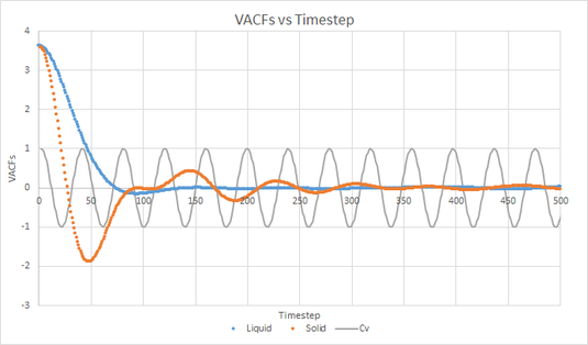
The velocity auto-correction function tells us about the dynamic processes within a system. If the atoms are not interacting with one another, they will retain their velocity for all timesteps (Newton's Law of motion) and the graph would simply be a horizontal line. Solids and liquids have strong inter-molecular forces due to the close packing of the atoms therefore producing more interesting VACF plots. In these phases the atoms arrange themselves in a position that will balance the repulsive and attractive forces between them, therefore it will minimize the energy of the system. The minima in the plots represents a collision between atoms .

Liquid (Blue curve)

The atoms do not have a fixed position but they are free to move throughout the system. The shape of the VACF curve is caused due to a collision between two atoms (the minima in the curve) followed by an oscillation around 0 which corresponds to the atoms having rebounded of one another and diffusing away from each other.

Solid (Orange curve)

In a solid the atoms are confined to a specific lattice coordinate and therefore cannot diffuse away. Instead a solids VACF plot oscillates around 0 as the atoms vibrate in their positions, the negative VACF value relating to a movement in the opposite direction of a positive value.

Harmonic Oscillator (Grey curve): The oscillations of the HO do not decay like they do in the solid and the liquid due to it considering only classical and not quantum effects. The LJ VACFs also take into account the whole system and plot an average - therefore as there are many atoms in the simulation their phases will 'cancel out' and lead to a decrease in oscillation magnitude, whilst this does not happen in the HO.

JC: Quantum effects are not included in the solid or liquid VACF either since the simulations are classical. The solid and liquid VACF decays to zero due to collisions between atoms which randomise the velocities and which are not present in the harmonic oscillator.

Task 4:

Use the trapezium rule to approximate the integral under the velocity autocorrelation function for the solid, liquid, and gas, and use these values to estimate in each case. You should make a plot of the running integral in each case. Are they as you expect? Repeat this procedure for the VACF data that you were given from the one million atom simulations. What do you think is the largest source of error in your estimates of D from the VACF?

Figure 25: Running integral for gas

Figure 26: Running integral of solid

Figure 27: Running integral of liquid

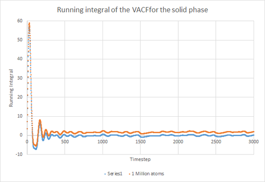
Solid, 32,000 atoms:

$D=-0.06665$

Solid, 1 Million atoms:

$D=0.528$

The negative diffusion coefficient is due to the value being so close to 0 due to the restricted movement of the atoms in the solid.

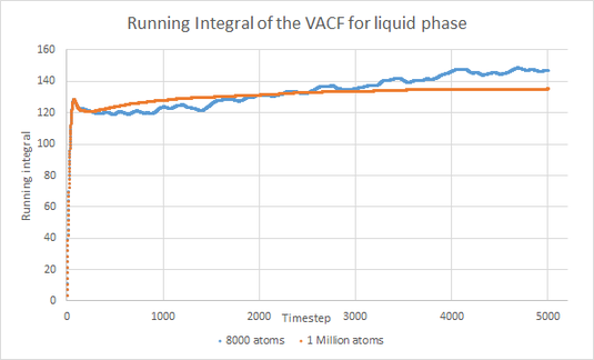
Liquid, 8,000 atoms:

$D=49.86$

Liquid, 1 Million atoms:

$D=45.05$

Gas, 8,000 atoms:

$D=2773.68$

Gas, 1 Million atoms:

$D=1635.43$

The diffusion coefficients follow the trend of decreasing in value from Gas > Liquid > Solid which is consistent with the trend obtained using the MSD calculation. The largest source of error is probably the use of the trapezium rule, a better choice would have been a Gaussian quadrature.