JC: General comments: All tasks answered correctly and good, clear and concise explanations of what your results show, well done. You could have added a bit more detail to your answers to the last sections on the RDF and dynamics.
By Charlie Farnham
Introduction to Molecular Dynamics Simulation
Molecular dynamics is the study of the physical movements of particles, using a computer simulation of a N-body simulation.[1] The method originated in the 1950s and 60s, pioneered by the physicists such as Metropolis and Fermi.[2][3] While Metropolis and his team had managed to simulate a liquid of imaginary 2D spheres, Fermi was seeking to model forces between neighbouring atoms as a function of time. This type of simulation is extremely important to modern science, a good example being its use in predicting the behavior of biological and drug molecules when in contact with receptors and other bio-molecules.[4] In this particular lab, use of the velocity-Verlet algorithm is employed to consider both starting positions and initial velocities of all atoms in a defined region. The significance of timestep values is explored and the Lennard-Jones interactions of pairs of atoms are considered to simulate and investigate real molecular dynamics.
Harmonic Oscillator Demonstration
Initially, this section analyses the discrepancy between modelling a classic harmonic oscillator when using the classic solution and when using the velocity-Verlet algorithm solution. The position at time t for a classic harmonic oscillator is given by the following equation:
Graph of absolute error between classic and Verlet algorithm solutions of position of a harmonic oscillator.
Looking at the blue absolute error graph above, it can be seen that the error oscillates between 0 and an ever increasing maximum. This is explained by considering that the classical and velocity-verlet solutions are themselves sine waves, that at given times, regardless of their phase will intercept (resulting in a discrepancy of 0 at that given time). Observing the orange error maxima trend line it can be seen that total error increases as a function of time. This is because the errors with each sequential calculation are accumulative.
JC: Good understanding.
Graph of position versus time for the displacement of a harmonic oscillator using classical solution.Graph of Total Energy versus time for the velocity-Verlet algorithm
It is expected that total energy, consisting of kinetic and potential energy would be constant. A fluctuation in potential energy is coupled with a fluctuation in kinetic energy, resulting in a constant total energy (as one energy decreases it is exchanged into the other). As seen in the graph above, the model is not perfect and there is a negligible fluctuation in total energy. Time step is the number that controls how many calculations are made in a given time. The smaller the time step and therefore the more calculations made in a given time, the more realistic the model but the more difficult the set of calculations. 0.20 is the larger time step that resulted in a maximum error of 1.005% about the average, actual energy value. A time step of 0.19 gave a maximum error 0f 0.904% about the average energy. Clearly, a time step value between 0.19 and 0.20 is required to limit total error to 1.00%. It's important to monitor the total energy of a physical system when modelling its behaviour numerically because energy in the real system should be conserved and this should be simulated as accurately as possible in the model.
JC: The Verlet algorithm is based on a Taylor expansion which is more accurate for a smaller timestep.
.This is shown in the two graphs below.
Graph of Energy versus time with time step 0.20Graph of Energy versus time with time step 0.19
A time step of less than 0.19 would of course reduce the percentage error, but this would be an unnecessary level of accuracy.
.
.
Atomic Forces
For a single Lennard-Jones Interaction, when the potential energy equals 0, the separation (r) is found as follows:
Since r0 or separation is larger than zero, we know that r0 equals positive sigma.
The force at this separation is found as follows:
The equilibrium separation and well depth are found as follows:
At equilibrium separation, force is set equal to zero.
The following integrals are evaluated when
This is probing to test at which separation, r, do we no longer consider an interaction between two atoms as significant. Of course, the force between two atoms decreases rapidly with r, and calculating this at infinite distance would be impossible to compute. (A cut off point must be decided, which is a compromise between simulating the real situation as closely as possible and allowing the computer to solve functions within a reasonable time).
JC: All maths correct and clearly laid out.
Periodic Boundary Conditions
1 mL of water equates to 0.056 moles. The total number of water molecules if therefore the product of the number of moles and Avogadro's constant: NA x 0.056 = 3.34 x 10²² molecules.
10000 molecules of water equate to 1.66 x 10⁻²⁰ moles. (10000/NA). 1 mole of water occupies 18 mL, so 10000 molecules occupy 2.99 x 10⁻¹⁹ mL.
Considering an atom at position (0.5,0.5,0.5) in a cubic simulation box running from (0,0,0) to (1,1,1). The atom moves along the vector (0.7,0.6,0.2) in a single time step. Without the boundary conditions, the atom would end up at position (1.2, 1.1, 0.7). The conditions mean that when an atom leaves the boundary, it is replaced by a replica atom entering from the opposite face of the boundary. After the periodic boundary conditions have been applied, it ends up at (0.2, 0.1, 0.7).
Reduced Units
To make values more manageable when using Lennard-Jones interactions, scaling factors are introduced, which convert real units into reduced units.
JC: Correct, but makes more sense to give r in nm.
Equilibration
Creating the Simulation Box
Giving atoms random starting coordinates is likely to cause problems with simulations. This is because many atoms are being generated within a limited space, meaning the likelihood of two atoms overlapping or being very close to each other is high. Looking at the Lennard-Jones equation, we can see that when the inter-nuclear distance is below the equilibrium distance, the energy of the interaction between the two atoms becomes dramatically larger and hence the accuracy of the simulation becomes questionable.
JC: With high repulsive forces the simulation will crash unless a much smaller timestep is used.
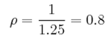
There is one lattice point per unit cell. Consider a unit cell with volume 1.077223 = 1.25. The number density specifies the number of lattice points per unit volume and is given by the equation p = n/V .
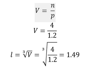
Considering a face centred cubic lattice with a lattice point number density of 1.2, the length of the side of the cubic unit cell can be calculated (n = 4 for a face centred cubic lattice).Using the original, simple cubic lattice, a simulated region of 10x10x10 unit cells contains 1000 atoms (as there is 1 atom/lattice point in each unit cell). If this were defined for the face centred cubic lattice with the same dimensions instead, it would be found that the region contained 4000 atoms, as each unit cell has 4 atoms/lattice points.
This code sets the mass of all atoms of type 1 to 1.0.
mass 1 1.0
For the next piece of syntax, style = one of a selection of pre-programmed styles, args = arguments used by the chosen style.
pair_style style args
This piece of code (pair_style) generally sets the formulas that describe pair wise interactions. Potentials between pairs of atoms are described only for pairs within a certain distance. Lennard Jones potential with no coulomb interactions is calculated using the text lj/cut. The global cut off for Lennard Jones interactions is set to 3.0 in this example.
pair_style lj/cut 3.0
For the final syntax, I,J = pair of atom types, args = coefficients for pairs of atom types.
pair_coeff I J args
The use of an asterisk ensures that the coefficients are set for multiple atom type pairs. This specific piece of code dictates how the atoms interact with one another and sets the force field coefficients to 1.0 for all atom types.
pair_coeff * * 1.0 1.0
JC: What are the force field parameters for this simulation, considering you are using a Lennard-Jones potential?
Given that we are specifying xi (0) and vi (0), we shall be using the velocity-Verlet integration algorithm. As discussed earlier, this algorithm considers both starting positions and initial velocities.
Running the Simulation
Looking at the lines of code below. The second line (variable timestep) ensures that if the text 'timestep' is encountered on any subsequent line, then the word 'timestep' should be replaced by the given value. In the example below, this value is always replaced by 0.001.
### SPECIFY TIMESTEP ###
variable timestep equal 0.001
variable n_steps equal floor(100/${timestep})
variable n_steps equal floor(100/0.001)
timestep ${timestep}
timestep 0.001

### RUN SIMULATION ###
 run ${n_steps}
 run 100000
This seems complex and begs the question, why not just simply write the following:
timestep 0.001
run 100000
The code ensures that the timestep remains at 0.001 throughout any simulation runs. The reason that the more complex version is used when setting the timestep as a variable is that when the value of timestep is manually changed for a new simulation, the number of steps (which is directly affected by the timestep) will be adjusted automatically without the need for manual input.
Checking Equilibration
The following graphs are plots for the timestep 0.001 of energy, temperature and pressure against time.
Graph of Energy vs Time for a Timestep of 0.001Graph of Pressure vs Time for a Timestep of 0.001Graph of Temperature vs Time for a Timestep of 0.001
.
All three graphs prove that the simulation reached equilibrium, showing a plateau in y values. Using a zoomed in version of the energy vs time graph, it can be seen that the system equilibrates at a time of approximately 0.3.
Zoomed in Version of 0.001 Timestep Energy vs Time graph
The graph below shows a comparison between the energy vs time graphs for all the different timesteps used.
The timesteps of 0.01 and 0.0075 are both acceptable, equilibrating at an energy of approximately -3.182 and both with equal fluctuation about the average value. The timesteps of 0.0025 and 0.001 are both slightly more acceptable, as they fluctuate by a lesser amount around an average, equilibrium energy value of about -3.185.
0.01 is the largest acceptable timestep, but 0.0025 would produce the most accurate results and still is, itself, a reasonable timestep for the length of simulation run in this experiment.
The timestep of 0.015 is a particularly bad choice because it, in fact, does not reach equilibrium (as seen below).
Graphs of Energy vs Time for All Timesteps
JC: The average total energy should not depend on the choice of timestep. 0.0025 has the same total energy as the smallest timestep so is the best choice.
Running Simulations Under Specific Conditions (Temperature and Pressure Control)
Thermostats and Barostats
From statistical thermodynamics, we can write the following two equations:
Generally, instantaneous temperature, T will fluctuate away from our target temperature. To ensure that temperature remains correct, i.e.:
each velocity value must be multiplied by gamma. We can then determine gamma by rearrangement.
JC: Correct.
Examining the Input Script
The following syntax is used to code for an averaging command, which takes a number of values and computes their average over a given number of timesteps.
Nevery = 100 = this instructs the computer to incorporate the input value at every 100th timestep into the average.
Nrepeat = 1000 = this instructs the computer to use each input value 1000 times when calculating an average.
Nfreq = 10000 = this instructs the computer to calculate an average at every 10000th timestep.
Values of temperature, etc will therefore be sampled at every 100th timestep.
Total number of timesteps divided by 100, will be the number of measurements that contribute to the average. Each measurement is contributed 1000 times.
Since the command reads 'run 100000', this number multiplied by the timestep 0.0025 will simulate 250 units of time.
Plotting the Equations of State
The graph below compares ideal gas behaviour to simulations ran at pressures of 2.5 and 3.0, with error bars included for both the x and y axis. The temperature used at each pressure were 1.5, 3.0, 4.5, 6.0 and 7.5 (inclusive of and above the critical temperature).
Graph of Density Against Temperature For Varying Pressures (Comparison also to ideal gas behaviour)
The simulated densities at each pressure are lower than the ideal gas law predicts. The ideal gas law essentially states that all interactions between the particles in a system are negligible and therefore not considered.[5] The densities are lower than in the ideal gas law prediction because the particles in the simulated liquid are interacting when they get too close and repelling each other via Lennard-Jones interactions. This causes the particles to spread out over a larger volume and therefore reduce the density.
The discrepancy between ideal gas law predictions and the simulation increases with increased pressure (at all temperatures tested), as can be seen in the table below. This happens because at high pressure the particles occupy a smaller volume and are therefore packed more closely together. Lennard-Jones interactions become more significant for the simulation at higher pressure and are still being ignored by the ideal gas law prediction. Hence, at higher pressure the discrepancy becomes larger due to inter-molecular interactions reducing the density of the simulated system.
Table Showing Discrepancy Between Simulated Density and Ideal Gas Density for Varying Pressure
The discrepancy between ideal gas law predictions and the simulation decrease with temperature. This is because as the kinetic energy of the particles increases, their movement begins to overcome repulsive inter-molecular interactions in the simulation. The inter-molecular interactions become more and more negligible. The simulation therefore mirrors the ideal gas behaviour more closely at higher temperatures.
JC: Good explanations of the different trends. Don't connect the simulation data points with a smooth line unless you are fitting the data points to a specific function.
Calculating Heat Capacities Using Statistical Physics
The graph below compares the effect of different densities (0.2 and 0.8) on the value of heat capacity/ volume for a range of temperatures (2.0, 2.2, 2.4, 2.6 and 2.8).
Graph of Heat Capacity/ Volume versus Temperature for Varying Densities
The general trend for both plots is that Cv/V decreases with temperature. Specific heat capacity is defined as the heat energy needed to increase the temperature of a given mass of a certain substance by one degree. As more heat energy is provided, higher energy states are occupied. With higher energy states, the energy difference to the next, higher state becomes smaller and smaller. This means the promotion to the next energy state requires less energy and the substance as a whole will require less heat energy to raise in temperature by a given amount (i.e. the heat capacity has decreased).
It can also be seen that the heat capacity of the substance increases with increased density. Increasing density increases the number of particles within the defined volume. This means that the same heat energy is shared across a larger number of particles and, hence the temperature is not raised as much as it would be at lower density with less molecules. This signifies that the heat capacity is larger for a higher density system, as the heat energy is spread over more particles.
It should be noted that there is a 'bump' in the trend for a density of 0.8. This could be for a number of reasons and requires further analysis to justify its presence. It can be speculated, however, that at a temperature of 2.4 this system contains particles with a particularly large density of states at a particular energy level. If this is the case, the heat capacity would increase producing a bump as seen above due to there being a larger requirement of heat energy to fill all energy states.
JC: Great explanation, as you say further work would be needed to confirm these conclusions.
Provided below is an example of the input scripts (for a density of 0.2 and temperature of 2.0).
Structural Properties and the Radial Distribution Function
Below is a graph containing plots of radial distribution against distance r for solid, liquid and gas phases. It shows how density of particles varies as a function of radial distance, r, away from the central atom concerned. The following input conditions were used:
Solid: density = 1.2, temperature = 1.0
Liquid: density = 0.8, temperature = 1.15
Gas: density = 0.07, temperature = 1.15.
Radial Distribution Functions Against Distance, r, for Solid, Liquid and Gas Phases
Similarities between phases:
At a small inter-molecular distance of r = 0 up until r = 0.9, all distribution functions produce a g(r) density value of 0. This is because the particles repel each other, so will not be found overlapping or in close proximity of one another.
All plots tend to 1 as infinity inter-nuclear distance r is approached, this value is the inherent density of the entire system.
JC: g(r) is normalised using the value of the bulk density.
Differences between phases:
The most noticeable difference between the phases is the trend in the number of peaks. Solid has the most peaks, then liquid and finally gas only has a single peak. The fact that the RDF for solid phase has many peaks over a long distance range shows that the system has long range order. A crystalline, solid structure possesses numerous particles at almost identical radial distances from the central particle. The first peak correlates to the particles nearest neighbours in the lattice and the second peaks to those the next distance, r, away and so on. The first peak is far sharper than the next peak at a larger distance. This is because the nearest neighbours will not vary much in their distance from the central particle, but this discrepancy in r between similar distanced particles will increase with distance from the central atom (hence widening the peaks). The solid also has sharper peaks than those of the gas and liquid phases, indicating the regularity of the solid structure and showing that the solid particles are trapped in a very small range of distance, r.
For the liquid phase, the peaks are not present for the same reason. Liquids can be thought of as particles surrounded by primary and secondary spheres of more liquid particles. The peaks become smaller and broader as the successive spheres of liquid particles become more diffuse and less confined. The peaks are less sharp than those of the solid phase, as the liquid particles are free to move more than those of the solid, meaning they are found over a wider range or r values (the r values are less discretised).
The gas phase plot reaches a radial distribution of 1 at the lowest value of r, as it is already very low in density. Its lack of peaks are due to the gas phase lacking in any repetition of structure or order.
Solid RDF Plot:
Illustration of Lattice Spacings for A Face Centred Cubic Lattice
Referring to the illustration above, the first three peaks correspond to the following lattice sites:
peak at r = 1.043 corresponds to site at distance b
peak at r = 1.475 corresponds to site at distance c
peak at r = 1.806 corresponds to site at farthest distance a.
The lattice spacings are:
b: (1/2, 1/2, 0) = 1.043
c: (0,1,0) = 1.475
a: (1/2, 1,1/2) = 1.806
JC: The lattice spacing is the distance between unit cells, in this case b, but you could have got a more accurate value for this by also expressing the distances to the first and third nearest neighbours in terms of the distance b, solving for b and then calculating an average value.
The coordination number for each of the three peaks is as follows:
b = 12
c = 6
a = 24
The integrals of the radial distribution function are included below:
Integrals of Radial Distribution Functions
JC: How did you calculate the number of nearest neighbours? Show the integral of g(r) at small r to show the number of nearest neighbours responsible for each peak.
Dynamical Properties and the Diffusion Coefficient
Below are the plots of mean squared displacement versus timestep for solid, liquid and gas phase small systems and systems containing 1 million atoms. These plots provide information on the displacement of a particle in a given time and due to this offer a chance to gather information about the system as a whole. If the graph levels off, this suggests that the particle is trapped at a certain displacement. A curved graph (only up as the y values are squared) indicates an external force acting on the particles. A straight line that isn't of gradient 0 shows that the particle is only experiencing the effects of diffusion.
JC: The curve at the beginning of these graphs indicates ballistic motion, when displacement is proportional to time, it is not due to an external force.
Graph of MSD versus timestep for Gaseous Systems possessing varying atom numberGraph of MSD versus timestep for Liquid Systems possessing varying atom numberGraph of MSD versus timestep for Solid Systems possessing varying atom number
These graphs are as expected. The simulations ran involved no applied force on the system or its particles. Therefore, as expected, a straight line graph is eventually produced for both the liquid and vapour plots. The liquid plot becomes linear faster than the gaseous plot.
The solid plot levels off, as expected. This is because in the crystal lattice, the solid system and its particles are locked in position. There are, however, slight fluctuations around the final MSD value due to particle vibration in the lattice. The MSD values are smallest for the solid, larger for liquid and largest for the gas. The explanation for this is obvious, the solid is denser and its particles are more confined than the gas and the liquid. The displacement values for the particles in a gaseous system will be larger as the particles have more kinetic/thermal energy.
Modelling the straight line section of each plot as follows and considering the gradient of the graphs to equal the 'm' part of the equation below allows the calculation of the diffusion coefficient, D. (all units were converted to real units).
Below is a table of the D values calculated. The million atom simulations all match closely to the smaller simulations. The solid simulations agree to the closest values. The liquids have similar values and the gas simulations have the largest discrepancy between values.
Table of D values
JC: What do you mean by real units? It would be good to show the lines of best fit that you used to calculate D on the graphs.
A second way to calculate D involves an equation called the velocity autocorrelation function. It is evaluated in terms of a 1 dimensional harmonic oscillator. After some lengthy integrations it is found that:
JC: The derivation can be simplified by using double angle formula to simplify the numerator and then identify this as an odd function to avoid having to perform the integration.
Below are plots of VACF against timestep for solid and liquid simulations, as well as for the harmonic oscillator function. This graph shows the average velocity of all particles. Therefore the minima in VACFs represent when a particle has become to close to another particle and begins to be repelled. The repulsion continues until the velocity of the particle becomes 0 and it then changes direction and moves away from the particle it has just 'collided' with. Eventually the simulations reach a point in time where all the velocities of all particles cancel out and the average velocity becomes 0.
This is not the case for the harmonic oscillator as this function models the velocity of a single particle. There are no particles to collide with, so the plot oscillates to infinity.
The liquid graph levels off faster than the solid graph. This is because there are more degrees of freedom for the particles in the liquid. Since their movement is less restricted they reach an equilibrium point faster, where the
velocities of each particle cancel out and the particles are more able to diffuse away from an interaction.
The solid particles are more restricted and confined in their crystal lattice, meaning the atoms aren't as free to reach the point so quickly where their average velocities equal 0.
Using the trapezium rule, the area under the VACF plots for the solid, liquid and gas phase are predicted. This allows a prediction of D to also be calculated using the following equation:
Integral
Trapezium Rule Prediction
D
Solid small system
-0.374744354000011
-0.12491
Solid 1 mil. Atoms
-0.374744354000011
-0.12491
liquid small system
123.737698410600000
41.2459
liquid 1 mil. Atoms
123.737698410600000
41.2459
gas small system
1299.701075000000000
433.2337
gas 1 mil. Atoms
490.153176500000000
163.3844
The only disparity in D value between the smaller simulation and that containing 1 million atoms, is for the gas phase. The trapezium rule is of course a large source of error as the area under the graph is approximated into discrete trapezoids. The expected running integrals we obtained.
JC: How did you use that equation? You should show the graphs of the running intergal. Did the graphs level off at long times, why is this important?
Conclusion
To conclude, molecular dynamics is a powerful tool for modelling chemical systems. It consists of useful tools such as radial distribution functions that can be used to accurately predict density of atoms at certain radial distances from a reference point.This investigation has only brushed the surface of liquid simulations and does not emphasize the significance of this computational method. From modelling protein interactions to assessing the affects of pressure on a super critical fluid, the applications of molecular dynamics are seemingly endless.
References
↑Alder. B. J, Wainwright. T. E, (1959), J. Chem. Phys, 31 (2), 459, doi: 10.1063/1.1730376
↑Fermi. E, Pasta. J, Ulam. S, (1955), Los Alamos report LA, doi: ACC0041.pdf
↑N. Metropolis, A.W.Rosenbluth, A.H. Teller, E. Teller, (1953), J. Chem. Phys.21, 1087, doi: 10.1063/1.1699114.