Talk:Cah12ls

JC: General comments: Well written report with some good explanations demonstrating a good understanding of the material. Try to check over your report before you submit it to make sure that all of the text is written as clearly as possible and that the figures are directly referred to in the text.

Liquid Simulations

Introduction to molecular dynamic simulations

The velocity-verlet algorithm models the behaviour of a classical harmonic oscillator and can be utilized to calculate the trajectories of particles in molecular dynamic simulations.

The classical solution to the total energy of a spring is the kinetic energy plus the potential energy and is given by the equation:

$E=\frac{1}{2}m{v}^2+\frac{1}{2}k{x}^2$

The formula used to calculate the position at time, t, for the classical harmonic oscillator is:

$x\left(t\right)=A\cos (\omega t+\varphi )$

The given initial conditions are:

k = 1.00 Timestep = 0.1000, Mass = 1.00, $\varphi$ = 0.00, A = 1.00, $\omega$ = 1.00

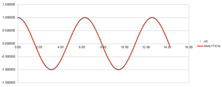
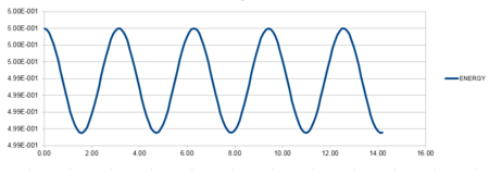
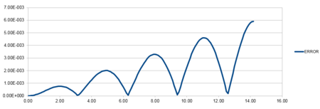
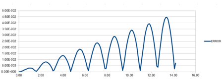
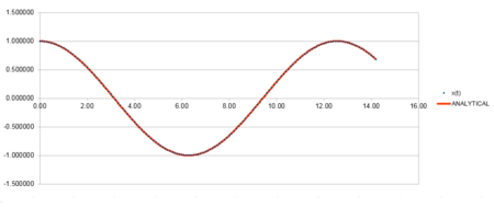
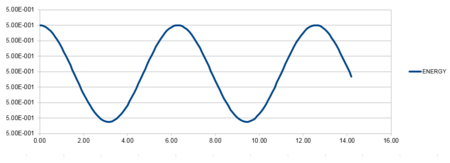
Position against time plot for the initial conditions	Energy against time plot for the initial conditions	Error for the energy against time plot

The position against time plot shows that the velocity-verlet algorithm is in good agreement with the energy calculated from the classical equation.

For a classical harmonic oscillator, the energy remains constant with time. The oscillations on the energy against time plot are between 0.4988 and 0.5000. The total energy fluctuation is approximately 0.30%, showing a good oscillating frequency indicative of the cosine curve. The minima and maximum values on the curve correspond to the pi, 2pi, 4pi etc maximum and minima on the cosine curve. Consequently, we can assume that the energy does indeed remain constant and therefore follows the first law of thermodynamics.

In addition, it can be shown that there is a relationship between mass, frequency of oscillation and k by the equation:

$\omega =\sqrt{\frac{k}{m}}$

Where k = force constant, m = mass and $\omega$ = frequency

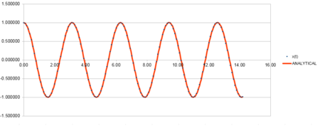
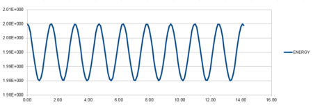
Which shows that as the force constant increases, the frequency of oscillation increases. This is due to an increased compression and therefore increased bounce back. The graphs below represent this and an arbitrary value of 4 was altered to display this relation.

Position against time plot for 4k	Energy against time plot for 4k	Error for the energy against time plot for 4k

The inverse is true for mass which shows a decrease in the frequency due to a decrease in the rate at which the particle on the spring can bounce back. Therefore the observed graphs will have a larger oscillation frequency. Again an arbitrary value of 4 was applied to the mass.

Position against time plot for 4m	Energy against time plot for 4m	Error for the energy against time plot for 4m

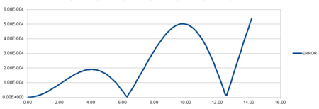
The line of best fit graph can be made by the estimate of the maximums in the error for the time step 0.01.

Error against time line of best fit

The accuracy of the position versus time graph is defined as the difference between the analytical and Velocity-Verlet solution for x(t).The line has a positive linear gradient and therefore shows that the error increases as time increases. This is due to the cumulative addition of the errors added each time because each change in position has an error associated with it and is calculated using the taylor expansion series which is summative.

After altering the timestep, it was measured that you need a timestep value of 0.211 to ensure that the total energy doesn't change by more than 1% (0.005) aka to ensure that the oscillations do not fluctuate beyond 0.495 and 0.505.

It is important to monitor the energy of a system when modelling behavior numerically because the first law of thermodynamics states that energy cannot be created or destroyed, merely transformed from one form to another. If the total energy were to change then this would lead to inaccurate results as the conservation of energy would not be obeyed upon application of the simulation. If there was a difference in the total energy then this indicates that the code in putted into the simulation may not be correct. Therefore if there is a change in energy, you may go back to the notepad script and re-write the code. For example, if the energy of the system increases as the simulation proceeds, then one may create a heat sink in the simulation to account for the access energy. This should then result in a simulation with no change in total energy.

JC: Good choice of timestep.

Atomic Forces

The Lennard-Jones potential is given by

$\varphi \left(r\right)=4ϵ(\frac{{\sigma }^{12}}{r^{12}}-\frac{{\sigma }^6}{r^6})$

When $r=r_0$ $\varphi \left(r\right)=0$

$0=4ϵ(\frac{{\sigma }^{12}}{r_0^{12}}-\frac{{\sigma }^6}{r_0^6})$

$0=\frac{{\sigma }^{12}}{r_0^{12}}-\frac{{\sigma }^6}{r_0^6}$

$\frac{{\sigma }^6}{r_0^6}=\frac{{\sigma }^{12}}{r_0^{12}}$

$r_0^6={\sigma }^6$

$r_0=\sigma$

From classical physics it follows that the force acting on an object is equal to the negative derivative of the potential:

$\mathbf{F}=-\frac{\mathrm{d}\varphi \left(\mathbf{r}\right)}{\mathrm{d}\mathbf{r}}$

Therefore subbing in for $\varphi \left(r\right)$:

$\mathbf{F}=-\frac{\mathrm{d}[4ϵ(\frac{{\sigma }^{12}}{r_0^{12}}-\frac{{\sigma }^6}{r_0^6})]}{\mathrm{d}\mathbf{r}}$

$\mathbf{F}=\frac{48ϵ{\sigma }^{12}}{r_0^{13}}-\frac{24ϵ{\sigma }^6}{r_0^7}$

Remembering that:

$r_0=\sigma$

$\mathbf{F}=\frac{48ϵ}{\sigma }-\frac{24ϵ}{\sigma }$

$\mathbf{F}=\frac{24ϵ}{\sigma }$

This is the force at separation at $r_0=\sigma$

To find the equilibrium separation, $r_{eq}$, you apply the assumption that the equilibrium separation is the separation at which the force is zero:

So, when: $r=r_{eq}$ $\mathbf{F}=0$

$\mathbf{F}=0=-\frac{\mathrm{d}[4ϵ(\frac{{\sigma }^{12}}{r_{eq}^{12}}-\frac{{\sigma }^6}{r_{eq}^6})]}{\mathrm{d}\mathbf{r}}$

$\frac{48ϵ{\sigma }^{12}}{r_{eq}^{13}}-\frac{24ϵ{\sigma }^6}{r_{eq}^7}=0$

$\frac{48ϵ{\sigma }^{12}}{r_{eq}^{13}}=\frac{24ϵ{\sigma }^6}{r_{eq}^7}$

$2{\sigma }^6=r_{eq}^6$

$r_{eq}=2^{1/6}\sigma$

Using this result we can figure out the well depth $\varphi \left(r_{eq}\right)$ by inserting the solution obtained for $r_{eq}$ into the the Lennard-Jones equation:

$\varphi \left(r\right)=4ϵ(\frac{{\sigma }^{12}}{2^2{\sigma }^{12}}-\frac{{\sigma }^6}{2{\sigma }^6})$

$\varphi \left(r\right)=4ϵ(\frac{1}{4}-\frac{1}{2})$

$\varphi \left(r\right)=-ϵ$

Evaluating the integrals $\underset{2\sigma }{\overset{\mathrm{\infty }}{\int }}\varphi \left(r\right)\mathrm{d}r$, $\underset{2.5\sigma }{\overset{\mathrm{\infty }}{\int }}\varphi \left(r\right)\mathrm{d}r$, and $\underset{3\sigma }{\overset{\mathrm{\infty }}{\int }}\varphi \left(r\right)\mathrm{d}r$ when $\sigma =ϵ=1.0$ gives:

$\underset{2\sigma }{\overset{\mathrm{\infty }}{\int }}\varphi \left(r\right)\mathrm{d}r$

$\varphi \left(r\right)=4ϵ(\frac{{\sigma }^{12}}{r^{12}}-\frac{{\sigma }^6}{r^6})$

$\underset{2\sigma }{\overset{\mathrm{\infty }}{\int }}4ϵ(\frac{{\sigma }^{12}}{r^{12}}-\frac{{\sigma }^6}{r^6})\mathrm{d}r$

When:

$\sigma =ϵ=1.0$

$\underset{2}{\overset{\mathrm{\infty }}{\int }}4(\frac{1}{r^{12}}-\frac{1}{r^6})\mathrm{d}r$

$4\underset{2}{\overset{\mathrm{\infty }}{\int }}(\frac{1}{r^{12}}-\frac{1}{r^6})\mathrm{d}r$

$4{(\frac{1}{5r^5}-\frac{1}{11r^{11}})}_2^{\mathrm{\infty }}=-2.48*10^{-2}$

$4{(\frac{1}{5r^5}-\frac{1}{11r^{11}})}_{2.5}^{\mathrm{\infty }}=-8.18*10^{-3}$

$4{(\frac{1}{5r^5}-\frac{1}{11r^{11}})}_3^{\mathrm{\infty }}=-3.29*10^{-3}$

An estimate of the number of water molecules in 1 ml of water under standard conditions can be given by the calculation below.

Given that the volume of 1 ml in dm³ is

$V=1ml=1c{m}^3=1*10^{-3}d{m}^3$

Under standard conditions of atmospheric pressure and temperature the density of water is given by:

$\rho =999.8kg{m}^{-3}=999.8*10^{-1}gc{m}^{-3}$

$\rho =\frac{m}{V}$

Therefore the mass of water is given by:

$m=999.8*10^{-1}g$

Consequently the number of moles of water in 1 ml:

$n=\frac{m}{M}$

$n=5.55*10^{-2}mo{l}^{-1}$

The total number of molecules can then be calculated:

$N=n{N}_A$ where N_A is Avogadro's number

$N=3.34*10^{22}$ molecules

Therefore, there are $3.34*10^{22}$ molecules of water in 1 ml of water under standard conditions.

The volume occupied by 10000 water molecules can also be determined:

Total number of molecules = $N=10000$

So the number of moles is given by:

$n=\frac{N}{N_A}$

$n=1.66*10^{-20}mo{l}^{-1}$

and the mass is equal to:

$m=nM$

$m=2.99*10^{-19}g$

Again, under standard conditions the density of water is:

$\rho =999.8kg{m}^{-3}=999.8*10^{-1}gc{m}^{-3}$

$V=\frac{m}{\rho }$

Therefore the volume is given by:

$V=2.99*10^{-19}$

The total volume occupied by 10000 water molecules is $2.99*10^{-19}ml$

Imposing boundary conditions, an atom moving from (0.5, 0.5, 0.5) along the vector (0.7, 0.6, 0.2) in a box which runs from (0. 0, 0) to (1, 1, 1) and ends up at (0.2, 0.1, 0.7).

When working with reduced units we can calculate several properties of a system.

If the Lennard-Jones cutoff = $3.2*0.34=1.09nm$

From previous calculations, the well depth = -ε, and therefore:

Well depth $=\frac{120*1.38*10-23*6.022*1023}{1000}=-0.997kJ/mol$

$T=\frac{T^{*}ϵ}{k_B}$

From Reduced Temperature = 1.5, and cancelling k_B,

Temperature = $120*1.5=180K$

JC: All maths and calculations correct and clearly laid out.

Equilibration

Giving atoms random co-ordinates in the simulations causes problems because there may be other atoms nearby that you have not taken into account. In this experiment there are approximately 8000 atoms and therefore there is a high probability that there will be overlapping potentials between the nearby atoms that you have not accounted for in the simulation code. This will result in a much larger potential energy and a less accurate result at the beginning of the simulation. This is due to the repulsion of the atoms with each other, the Lennard-Jones potential increases as the internuclear distance between the atoms becomes smaller than its equilibrium distance, this relationship is seen by the Lennard-Jones equation in the previous section. This means there will be a large kinetic energy due to a fast movement of atoms on repulsion and consequently the timestep would need to be very small to observe these fast moving interactions.

JC: Good explanation, using a starting configuration with high repulsive forces can cause a simulation to crash unless a much smaller timestep is used.

Therefore in the simulation the atoms are placed on the lattice points of a cubic lattice.

To satisfy myself that the lattice spacing corresponds to a number density of 0.8, I will carry out the following numerical reasoning.

The volume of a cube is given by r³

Therefore the volume is equal to

$(1.07722{)}^3=1.25$

and the density is equal to the number of atoms divided by the volume

$\frac{1}{1.2500}=0.8$

The side length of a cubic unit cell with lattice point number density of 1.2 is given by the number of atoms per unit cell divided by the volume.

So the number of atoms is 4 per face centered cubic lattice and the density is 1.2, therefore the volume is given by

$\frac{4}{V}=1.2$

$V=\frac{4}{1.2}=3.333$

Therefore if you cube root this answer you get the length of one side (due to the volume being the length of one side cubed, so this is the inverse)

$r=3.333^{1/3}=1.4938$

The number of atoms per unit cell is 4, therefore if you had 1000 unit cells you would have 4000 atoms.

JC: Correct.

The purpose of the following input script is given below:

mass 1 1.0
pair_style lj/cut 3.0
pair_coeff * * 1.0 1.0

The 'mass 1 1.0' is the mass of the atom, where the specific atom type can be denoted I. So in this case there is just one type of atom in the simulation. If there were two different types of atoms the notation would now be mass 2 1.0. If there is no atom type specified and only an asterix is denoted then this means that the atoms from atoms 1 to N (where N is the maximum number of atoms types) all have the same mass which can be found in the 'value' section of the command. The position of the asterix denotes different things in the commands. If the asterix is before the n value, then this indicates that all atom types from 1 to n (inclusive) will have the mass defined by the value section of the command. If the asterix is after the n value, all atom types from n to N (inclusive), will have same value for the mass which is listed in the ‘value’ section of the command. If the asterix is inbetween all types from m to n then this means all atoms between the those two atoms will have the same mass value denoted by the value selection of the command.

The 'pair_style lj/cut 3.0' is used to calculate the pairwise interactions. This means that the pair potentials are defined between the two atoms before the 'cut-off' distance, which in this case is 3.0. The lj part defines the cut-off lennard-jones potential, the potential where there are no coulombic interactions. If there was no cut-off value then there would be an infinite number of potential pair interactions, leading to long simulation times and an inaccurate result.

The pair_coeff * * 1.0 1.0 is the pairwise force field coefficients for one or more pairs of atom types. The 1.0 1.0 values can be denoted I and J args respectively. These represent atom types, in this case both atoms are type 1, and args represents the coefficients for the atom types.

JC: In the pair_coeff command the asterisks specify the atoms types and the values of 1.0 are the pair coefficients for the interaction between those atom types. For the Lennard-Jones potential the pair coefficients are epsilon and sigma.

Due to the fact that we are specifying the Xi(0) and Vi(0), we use the velocity-verlet algorithm. This is because it assumes that the acceleration is independent of velocity and therefore we can calculate the individual atoms velocities.

The lines below are specifically written like this.

### SPECIFY TIMESTEP ###
variable timestep equal 0.001
variable n_steps equal floor(100/${timestep})
variable n_steps equal floor(100/0.001)
timestep ${timestep}
timestep 0.001

### RUN SIMULATION ###
run ${n_steps}
run 100000

This is because writing the code in this way (using the $ sign) means that this specific timestep can be included in every simulation. If it was written in the simplified version then you would have to input each timestep manually to keep the simulation running at a constant rate. Consequently, if we change the timestep duration, then the program will automatically alter the number of steps to be run to ensure it is still run in the same amount of time.

JC: Explanation is correct, but a bit unclear.

Resolution Trajectory	Resolution Trajectory of a single particle

Checking Equilibration

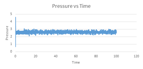
Energy vs time for timestep 0.001	Temperature vs time for timestep 0.001	Pressure vs time for timestep 0.001

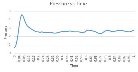
The graphs above show that the system reached equilibrium at approximately 0.3 seconds and this can be seen by the zoomed in versions on the graph below. This was determined by the fact that each property fluctuated around the same property value after 0.3.

Energy vs time for timestep 0.001 Zoomed	Temperature vs time for timestep 0.001 Zoomed	Pressure vs time for timestep 0.001 Zoomed

JC: Good idea to look at the beginning of the simulation to see how the properties approach equilibrium.

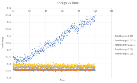
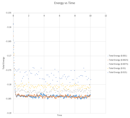
A combined plot of the total energy against time can be seen below for each timestep value.

Energy vs time for varying timestep

This shows that choosing different timestep values produces different results. On first look at the graph it looks as though the shorter the time step, the more accurate the result due to an equilibrium value being obtained. This however is not always an accurate way of evaluating simulations which run for long periods of time and therefore a balance between the timestep being accurate and the timestep observing the reaction is required. If you zoom in on the graph by looking at a shorter time frame you can see that the shorter times 0.0025 and 0.0075 do indeed produce a more accurate result as both reach an equilibrium, fluctuating around an average value more closely than the larger timestep values.

Energy vs time for varying timestep in a shorter time

It can also be noted from the graph above that the timestep of 0.0015 is not a good choice for this simulation. This is because there is a large variance between the values obtained and an energy equilibrium does not appear to have been achieved.

JC: Which timestep did you choose in the end? Why are the timesteps of 0.0075 and 0.01 not good choices even though the energy appears to fluctuate around a constant value - should the total energy of a simulation depend on the timestep?

Running simulations under different conditions

Changing ensemble

Five temperatures were chosen above the critical temperature of 1.5; 2, 2.5, 3, 3.5 and 4. They were chosen above this temperature to avoid the formation of a liquid-gas equilibrium, which would not produce accurate results. These were all then run at two different pressures 2.5 and 2.75. Those specific pressure values were obtained because this is the approximate equilibrium value that could be seen on the pressure against time graph in the previous section. A timestep value of 0.001 was used as this appeared to produce accurate results around an equilibrium value when used previously.

$\gamma$ is the constant factor we increase the velocity by to change the temperature. We want the temperature$T=\mathfrak{𝔗}$ with each fluctuation and therefore multiply every velocity by $\gamma$. Therefore we can calculate $\gamma$ starting with the two equations:

$\frac{1}{2}\sum _i{m}_i{v}_i^2=\frac{3}{2}N{k}_{B}T$

$\frac{1}{2}\sum _i{m}_i{\left(\gamma v_i\right)}^2=\frac{3}{2}N{k}_B\mathfrak{𝔗}$

Adding theses together results in:

$\frac{1}{2}\sum _i{m}_i{v}_i^2+\frac{1}{2}\sum _i{m}_i{\left(\gamma v_i\right)}^2=\frac{3}{2}N{k}_{B}T+\frac{3}{2}N{k}_B\mathfrak{𝔗}$

Since $\gamma$ is a constant, it can be taken out of the sum term:

$\frac{1}{2}\sum _i{m}_i{v}_i^2+\frac{1}{2}{\gamma }^2\sum _i{m}_i{v}_i^2=\frac{3}{2}N{k}_B(T+\mathfrak{𝔗})$

$\frac{1}{2}(1+{\gamma }^2)\sum _i{m}_i{v}_i^2=\frac{3}{2}N{k}_B(T+\mathfrak{𝔗})$

$(1+{\gamma }^2)\sum _i{m}_i{v}_i^2=3N{k}_B(T+\mathfrak{𝔗})$

Inserting for:

$\sum _i{m}_i{v}_i^2=3N{k}_{B}T$

Gives:

$3N{k}_{B}T(1+{\gamma }^2)=3N{k}_B(T+\mathfrak{𝔗})$

$(1+{\gamma }^2)T=T+\mathfrak{𝔗}$

$T+{\gamma }^{2}T=T+\mathfrak{𝔗}$

${\gamma }^{2}T=\mathfrak{𝔗}$

${\gamma }^2=\frac{\mathfrak{𝔗}}{T}$

$\gamma =\sqrt{\frac{\mathfrak{𝔗}}{T}}$

JC: Correct.

The three numbers 100, 1000, 100000 are important in the simulation because they tell you how the average of each thermodynamic property is calculated. It will appear in this format in the script:

 fix aves all ave/time 100 1000 100000 v_dens v_temp v_press v_dens2 v_temp2 v_press2 v_etotal       v_etotal2 

 run 100000

This command tells the LAMMPS program to take 100 timesteps, to take a total of 1000 samples and to repeat this until 100000 timesteps have passed. An average of each of the properties you are interested in (such as density, pressure, temperature, dens^2, temp^2, etotal, and etotal^2) is also then determined. So in summary, the first number is how many sample steps to take, the second is how many samples are taken in total and the third number is how long the sample runs for. In addition, increasing the simulation time will increase the number of averages that are generated. Since the timestep is 0.001 and we are simulating 100000 data points, we will simulate 100 reduced time units.

The ideal gas law is given by

$pV=N{k}_{B}T$

Which rearranging for the number density $\frac{N}{V}$ gives:

$\frac{N}{V}=\frac{p}{k_{B}T}$

When performing calculations with reduced units, $k_B$ takes a value of 1, therefore the above equation becomes:

$\frac{N}{V}=\frac{p}{T}$

The results obtained from the LAMMPS simulation and the results calculated using the ideal gas law are compared on the graph below.

Number density vs temperature for varying pressure

The graphs above show that the simulated value for density at each pressure was lower than the density calculated using the ideal gas equation. This may be explained by the fact that in the ideal gas equation you are assuming the potential energy of the system is zero, consequently there are shorter equilibrium distances between the atoms. However for simulated systems density has taken into account the repulsive Lennard-Jones potential term leading to larger internuclear distances; this results in lower densities.

In addition, the density calculated from the simulation has a better line of fit the higher the temperature due to an increase in temperature resulting in a higher mean free pathway and therefore fewer collisions per timestep and a lower potential energy (which then becomes similar to that described by the ideal gas law).

Also, increasing the pressure in both the simulated system and the ideal system increases the number density and the discrepancy between the ideal and simulated data also increases. A third pressure was calculated to confirm this trend. At the lower pressures the shapes of the curves for the simulated data are similar in shape to the curves for the ideal gas calculated data. This may be explained by the fact that the ideal gas assumes there are no intermolecular interactions. At lower pressures atoms are further apart and therefore less likely to interact. Consequently, the atoms behave 'more ideally' at lower pressures, so the simulated graphs will be of similar shape to those calculated using the ideal gas law.

Furthermore, it can be seen by the graph above that for all data, increasing the temperature decreases the number density. This may be explained by the fact that at high temperatures the molecules have a higher kinetic energy and are moving faster. This means there are fewer intermolecular interactions and therefore, in the case of the simulated molecules, they behave more ideally. Hence all the lines converge more closely at higher temperatures and there are fewer discrepancies.

Further investigation may be conducted to confirm trends between the simulated data and the ideal gas law by comparing the results to that predicted by the Van Der Waals equation; a different form of the ideal gas equation which now takes into account the potential energy of the system by assuming the atoms behave like hard spheres.

JC: Good explanations of the trends with temperature and pressure and good suggestion to use the Van der Waals equation to improve the agreement with the simulation results.

Calculating heat capacities using statistical physics

Ten phase point simulations were run; each density of 0.2 and 0.8 were run at the temperature values 2.0, 2.2, 2.4, 2.6 and 2.8.

The npt file code was altered so that it can carry out the simulation in density-temperature phase space rather than pressure-temperature phase space. An example input script of a density of 0.2 and a temperature of 2.0 is seen below:

 ### DEFINE SIMULATION BOX GEOMETRY ###

variable density equal 0.2
lattice sc ${density}
region box block 0 15 0 15 0 15
create_box 1 box
create_atoms 1 box

### DEFINE PHYSICAL PROPERTIES OF ATOMS ###
mass 1 1.0
pair_style lj/cut/opt 3.0
pair_coeff 1 1 1.0 1.0
neighbor 2.0 bin

### SPECIFY THE REQUIRED THERMODYNAMIC STATE ###
variable T equal 2.0
variable timestep equal 0.0025

### ASSIGN ATOMIC VELOCITIES ###
velocity all create ${T} 12345 dist gaussian rot yes mom yes

### SPECIFY ENSEMBLE ###
timestep ${timestep}
fix nve all nve

### THERMODYNAMIC OUTPUT CONTROL ###
thermo_style custom time etotal temp press
thermo 10

### RECORD TRAJECTORY ###
dump traj all custom 1000 output-1 id x y z

### SPECIFY TIMESTEP ###

### RUN SIMULATION TO MELT CRYSTAL ###
run 10000
unfix nve
reset_timestep 0

### BRING SYSTEM TO REQUIRED STATE ###
variable tdamp equal ${timestep}*100
variable pdamp equal ${timestep}*1000
fix nvt all nvt temp ${T} ${T} ${tdamp}
run 10000
reset_timestep 0

### MEASURE SYSTEM STATE ###
thermo_style custom step etotal temp atoms
variable temp equal temp
variable etotal equal etotal
variable etotal2 equal etotal*etotal
fix aves all ave/time 100 1000 100000 v_temp v_etotal v_etotal2
unfix nvt
fix nve all nve
run 100000

variable avetemp equal f_aves[1]
variable avetemp2 equal f_aves[1]*f_aves[1]
variable e2bracket equal f_aves[3]
variable ebracket2 equal f_aves[2]*f_aves[2]
variable cv equal atoms*atoms*(${e2bracket}-${ebracket2})/${avetemp2}
variable volume equal vol
variable cvv equal ${cv}/${volume}

print "Averages"
print "--------"
print "Density: ${density}"
print "AveTemperature: ${avetemp}"
print "HeatCapacity: ${cv}"
print "Volume: ${volume}"
print "HeatCapacityOverVolume: ${cvv}"

Isochoric heat capacity over volume vs temperature

The trend is as expected; the lower the density of the system, the lower the isochoric heat capacity over volume value. This can be seen that the density of 0.2 has an overall lower heat capacity compared to a density of 0.8. This may be explained by the fact that heat capacity is an extensive property, its value is proportional to the size of the system; the larger the system, the greater the heat transfer is required to achieve the same temperature change and therefore the greater the heat capacity. In the case of this system, if the volume was the same for both densities, the density of 0.8 will have more particles occupying the same space and therefore have a higher heat capacity.

In addition, as temperature increases, the isochoric heat capacity over volume value decreases. This may be explained by the fact that, according to boltzmann's distribution, the higher the temperature, the greater the number of accessible energy levels. As you move towards the higher energy levels they begin to converge and consequently the energy required to populate them decreases, and therefore a lower heat capacity is required.

JC: Good understanding, more analysis beyond the scope of this experiment would be needed to understand the trend with temperature in more detail.

Structural properties and the radial distribution function

Radial distribution functions $g(r)$ allow us to characterise the structure of systems such as the distance from an atom at which we will find it's nearest neighbour. Consequently, it can be used to determine the structural properties of the system. Below I have calculated the radial distribution function for the solid, liquid, and vapour phases of the Lennard-Jones fluid in a face centred cubic lattice.

Using the paper by Jean-Pierre Hansen and Loup Verlet, values for the density and temperature of each phase were estimated as:

Vapour: Density = 0.05, Temperature = 1.25

Liquid: Density = 0.8, Temperature = 1.25

Solid: Density = 1.1, Temperature = 1.25

The plot of each function is seen below.

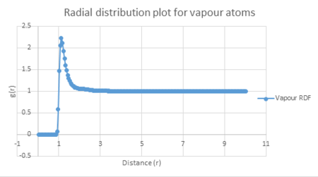
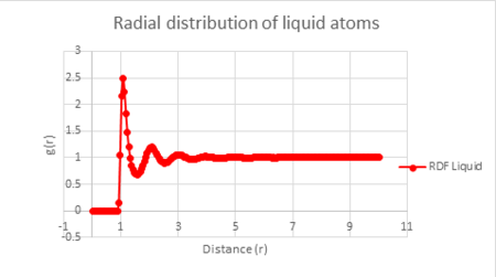
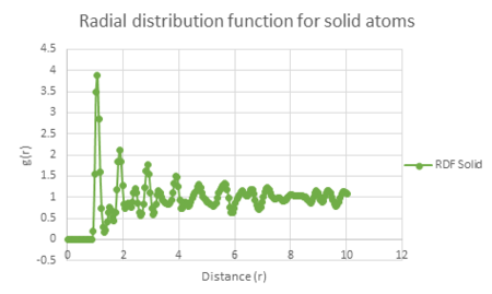
Vapour g(r) vs distance	Liquid g(r) vs distance	Solid g(r) vs distance

The three graphs above all show a radial distribution function of zero between a distance of zero and 1.075. This may be explained by the fact that at such short distances, the atoms will have high potential overlap and therefore large repulsive potentials. Consequently this means that the atoms cannot approach each other within this small distance.

The radial distribution function for the solid has the largest fluctuations of the three states. This may be explained by the fact that the position of the atoms in a solid are in a fixed lattice moving only with small vibrational motion. This means that you can easily observe the radial distribution of each atom relative to its neighbour due to this regular spacing.

The radial distribution function for liquids has fewer fluctuations than that for a solid, but more than for a vapour. This is due to the motion of atoms in a liquid following the random Brownian motion and therefore do not have exact positions in space like you find in a solid, but have a reduced movement in space compared to a vapour. Consequently, at short internuclear distances you can observe well defined peaks, whereas they become less well defined at long range distances. The three distinct peaks in the liquid radial distribution function show that this short range order is only observed between its three nearest neighbours.

The radial distribution function for vapour has only one peak. This shows that its system has a low degree of ordered molecules as the travel in a completely random motion. Therefore vapour does not display either short range order, like liquids and solids do, or long range order, like solids do.

JC: Good description of the different RDFs.

Radial distribution of all states g(r) vs distance

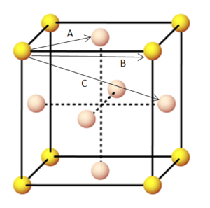
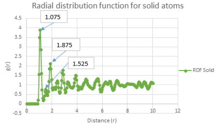
The shortest three interatomic distances within the face centred cubic lattice can be calculated using the radial distribution function against distance graph. The shortest distance corresponds to the first peak in the RDF (A on the face centred cubic diagram below). The second shortest distance corresponds to the second peak in the RDF (B). Finally the third shortest interatomic distance is associated with the third peak in the RDF (C). Their actual lengths can be seen by the labelled graph below.

Face centred cubic lattice

Radial distribution function of the solid system labelled - g(r) vs distance

This shows that A = 1.075 B = 1.525 C = 1.875.

The lattice spacing between the atoms can be seen by the value of B because in a face centred cubic lattice the second nearest neighbour is located exactly one lattice parameter away. Previously it was calculated that the lattice spacing for a face centred cubic is 1.494. The simulated value is greater than the theoretical value calculated, this may be because the density used in this simulation was 1.1, yet we had previously calculated the lattice spacing using a density of 0.8.

JC: Did you calculate the lattice parameter from the first or third peak as well? You could have calculated an average lattice parameter using the first three peaks rather than just considering the second peak.

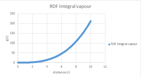
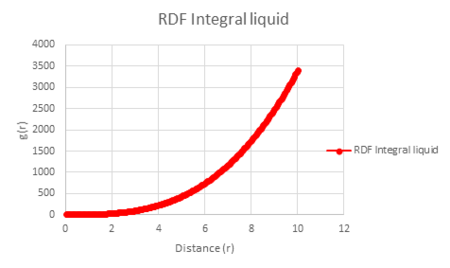
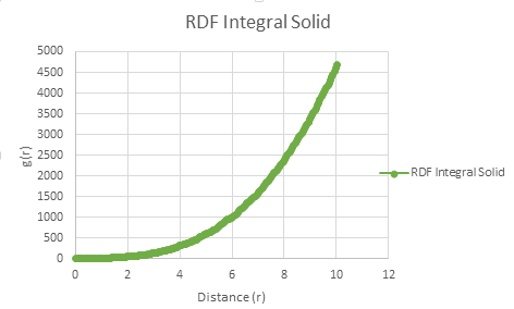
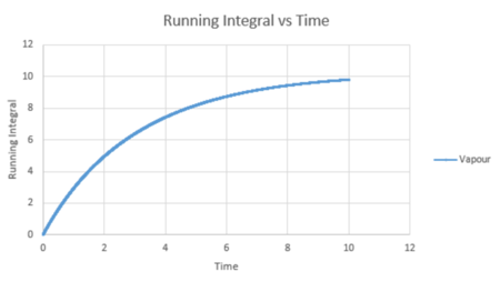
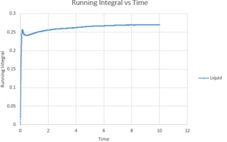
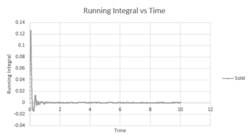
The coordination number for each of the first three peaks was obtained by looking at the running integral against distance diagram for the solid.

Vapour g(r) vs distance integral	Liquid g(r) vs distance integral	Solid g(r) vs distance integral

Radial distribution of solid running integral - g(r) vs distance

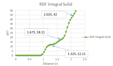
From the running integral graph the coordination number of the first nearest neighbour is found by looking at the value of r where the peak first diminishes. This is at 1.325 and has a running integral value of 12.11. The second peak diminishes at a distance of 1.675 and a value of 18.11. The final peak diminishes at 2.025 with a running integral value of 42. Therefore, the co-ordination of the first atom is 12. If you take the distance between the first two peaks (18.11-12.11) you get the value of the coordination of the second atom which is 6. Therefore the third nearest neighbour has an approximate coordination number of 24 (42-18.11).

Face centred cubic nearest lattice points

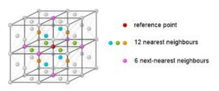
This can be confirmed by looking at the coordination environment of a face centred cubic in the picture above. It can be seen that the reference atom has 12 nearest neighbours, and then the next nearest neighbours has 6, after this are another 6 atoms which corresponds to the 24 coordination. Therefore the calculated coordination numbers agree with that observed by the crystal lattice.

JC: Great diagram to show that the numbers of nearest neighbours calculated from the RDF agree with the number for a perfect fcc lattice.

Dynamical properties and the diffusion coefficient

Mean squared displacement

The diffusion coefficient allows us to determine how much each atom moves around within the simulation. There are two different ways of calculating it; the mean squared displacement approach or the velocity autocorrection function approach.

To evaluate the mean squared displacement approach simulations were run at each state, solid, liquid and vapour. These were then used to calculate the diffusion coefficients using the equation below.

$D=\frac{1}{6}\frac{d<r^2(t)>}{dt}$

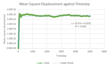
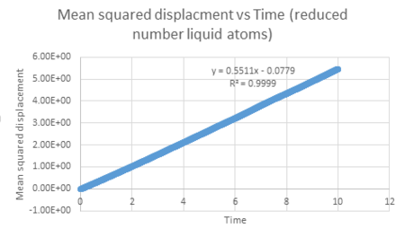
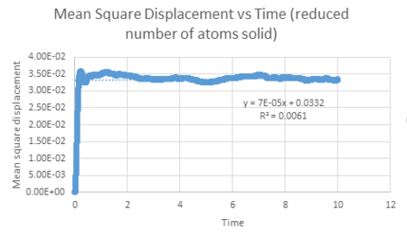
Vapour MSD vs timestep	Liquid MSD vs timestep	Solid MSD vs timestep

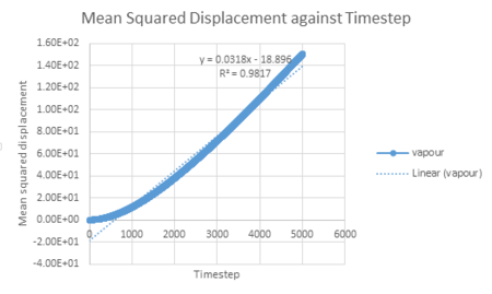
For the mean square displacement against time diagram obtained for vapour, the R squared value is 0.9817. This is beacuse the small timestep of 0.002 means that the data points at the start of the simulation follow a quadratic system rather than a linear system, this is called the ballistic regime. This may be explained by the fact that at the start of the simulation the vapour atoms are far apart and will therefore not collide, resulting in each atom having a constant velocity. This means that r, the distance travelled, is proportional to time. Therefore because the MSD is proportional to time squared, we observe a quadratic relationship at the start of the simulation aka parabolic behaviour. Once the graph becomes linear after a certain distance, we can observe the now expected browninan motion of the atoms; the linear relationship between timestep and the mean squared displacement.

For the mean square displacement against time graph obtained for the liquid the r squared value is 0.9999. This shows that there is a definite linear relationship between timestep and mean squared displacement for liquids due to the Brownian motion of the atoms. Liquids therefore differ from vapour because they do not show quadratic behaviour.

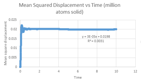
The mean squared displacement against time graph for a solid shows a very small r squared value, indicating that there is virtually no relation between mean squared displacement and timestep. This is to be expected due to atoms in a solid having fixed positions in space with small lattice vibrations. Also, there is a steep jump not long after the zero timestep, reaching a MSD value that has small fluctuations. This may be explained by the fact that once the solid atom has been displaced exploring its limited surrounding area, there is no further displacement.

JC: Good explanations.

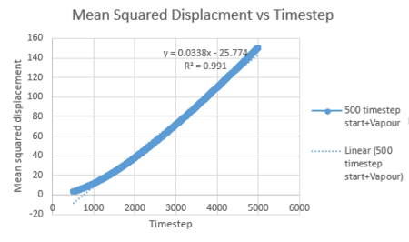
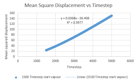
To minimise the effects of the quadratic effects on the linear trendline, the data can be evaluated over a different rate of timestep values. The graphs below show that the relationship becomes more linear (r squared moves closer to the value of 1) the smaller the timestep range for vapour.

Vapour MSD vs Timestep range 500-5000	Vapour MSD vs Timestep range 1000-5000	Vapour MSD vs Timestep range 1500-5000

Vapour MSD vs timestep for a million atoms	Liquid MSD vs timestep for a million atoms	Solid MSD vs timestep for a million atoms

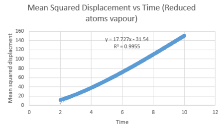
Vapour MSD vs time for the linear section of the graph	Liquid MSD vs time for the linear section of the graph	Solid MSD vs time for the linear section of the graph

Vapour MSD vs time for the linear section of the graph	Liquid MSD vs time for the linear section of the graph	Solid MSD vs time for the linear section of the graph

JC: The plot labelling is a bit unclear, give each plot a figure number so that you can refer to it directly in the text.

The diffusion coefficient can be calculated using the slope of the linear line for each graph of mean square displacement against time (where timestep has been converted to time by the time step 0.002). This value was divided by six to give the diffusion coefficient. The table below summarises the diffusion coefficients for all graphs.

	Diffusion coefficient for the system with reduced number of atoms (cm2s-1)	Diffusion coefficient for the million atom system (cm2s-1)
Vapour system	2.95	2.83
Liquid system	0.091	0.524
Solid system	1.17*10-5	5*10-6

JC: Are you diffusion coefficients really in cm^2 s^-1, what units is the mean squared displacement in?

In comparison to the million dollar system, we observe similar trends. This shows that increasing sample size does not significantly affect the overall results when calculating simulations. The diffusion coefficient is largest for vapour and is the smallest for solid in both cases. This is expected due to the random motion of vapour being greater than that of a solid and so can diffuse further. In addition, the solid has a negative gradient which may be due to an error calculated by the simulation program, highlighting that not all simulations can be deemed accurate.

Velocity Autocorrelation Function

To evaluate the normalised velocity autocorrection function for a 1D harmonic oscillator, we start with the position $x(t)$ for a classical harmonic oscillator equation:

$x=Acos(\omega t+\varphi )$

Differentiating the above equation using the chain rule gives:

$y=Acosu$ where $u=\omega t+\varphi$

$\frac{dy}{du}=-Asinu$ and $\frac{du}{dt}=\omega$

$\frac{dy}{dt}=\frac{dy}{du}\frac{du}{dt}$

$\frac{dy}{dt}=-A\omega sin(\omega t+\varphi )$

So:

$\frac{dx}{dt}=v(t)=-A\omega sin(\omega t+\varphi )$

Similarly, when $t=t+\tau$ we can apply the same method to differentiate the equation:

$x=Acos[\omega (t+\tau )+\varphi ]$

To obtain:

$v(t+\tau )=-A\omega sin(\omega t+\omega \tau +\varphi )$

Inserting the equations for $v(t)$ and $v(t+\tau )$ into the equation:

$C\left(\tau \right)=\frac{\underset{-\mathrm{\infty }}{\overset{\mathrm{\infty }}{\int }}v\left(t\right)v(t+\tau )\mathrm{d}t}{\underset{-\mathrm{\infty }}{\overset{\mathrm{\infty }}{\int }}{v}^2\left(t\right)\mathrm{d}t}$

Gives:

$C(\tau )=\frac{\underset{-\mathrm{\infty }}{\overset{\mathrm{\infty }}{\int }}A\omega sin(\omega t+\varphi )A\omega sin[\omega t+\omega \tau +\varphi ]\mathrm{d}t}{\underset{-\mathrm{\infty }}{\overset{\mathrm{\infty }}{\int }}A\omega sin(\omega t+\varphi )A\omega sin(\omega t+\varphi )\mathrm{d}t}$

Simplifying:

$C(\tau )=\frac{\underset{-\mathrm{\infty }}{\overset{\mathrm{\infty }}{\int }}sin(\omega t+\varphi )sin[\omega t+\omega \tau +\varphi ]\mathrm{d}t}{\underset{-\mathrm{\infty }}{\overset{\mathrm{\infty }}{\int }}si{n}^2(\omega t+\varphi )\mathrm{d}t}$

From the trigonometric identities it follows that:

$sin(u+v)=sin(u)cos(v)+cos(u)sin(v)$

So:

$sin(\omega t+\omega \tau +\varphi )=sin(\omega t)cos(\omega \tau +\varphi )+cos(\omega t)sin(\omega \tau +\varphi )$

Thus, applying this trigonometric identity to the function $C(\tau )$ leads to:

$C(\tau )=\frac{\underset{-\mathrm{\infty }}{\overset{\mathrm{\infty }}{\int }}sin(\omega t+\varphi )[sin(\omega \tau )cos(\omega t+\varphi )+cos(\omega \tau )sin(\omega t+\varphi )]\mathrm{d}t}{\underset{-\mathrm{\infty }}{\overset{\mathrm{\infty }}{\int }}si{n}^2(\omega t+\varphi )\mathrm{d}t}$

Multiplying out each term:

$C(\tau )=\frac{\underset{-\mathrm{\infty }}{\overset{\mathrm{\infty }}{\int }}sin(\omega t+\varphi )sin(\omega \tau )cos(\omega t+\varphi )+si{n}^2(\omega t+\varphi )cos(\omega \tau )\mathrm{d}t}{\underset{-\mathrm{\infty }}{\overset{\mathrm{\infty }}{\int }}si{n}^2(\omega t+\varphi )\mathrm{d}t}$

Separating the single integral into two integrals:

$C(\tau )=\frac{\underset{-\mathrm{\infty }}{\overset{\mathrm{\infty }}{\int }}sin(\omega t+\varphi )sin(\omega \tau )cos(\omega t+\varphi )\mathrm{d}t}{\underset{-\mathrm{\infty }}{\overset{\mathrm{\infty }}{\int }}si{n}^2(\omega t+\varphi )\mathrm{d}t}+\frac{\underset{-\mathrm{\infty }}{\overset{\mathrm{\infty }}{\int }}si{n}^2(\omega t+\varphi )cos(\omega \tau )\mathrm{d}t}{\underset{-\mathrm{\infty }}{\overset{\mathrm{\infty }}{\int }}si{n}^2(\omega t+\varphi )\mathrm{d}t}$

Taking out $sin(\omega \tau )$ and $cos(\omega \tau )$ from the integrals:

$C(\tau )=\frac{sin(\omega \tau )\underset{-\mathrm{\infty }}{\overset{\mathrm{\infty }}{\int }}sin(\omega t+\varphi )cos(\omega t+\varphi )\mathrm{d}t}{\underset{-\mathrm{\infty }}{\overset{\mathrm{\infty }}{\int }}si{n}^2(\omega t+\varphi )\mathrm{d}t}+\frac{cos(\omega \tau )\underset{-\mathrm{\infty }}{\overset{\mathrm{\infty }}{\int }}si{n}^2(\omega t+\varphi )\mathrm{d}t}{\underset{-\mathrm{\infty }}{\overset{\mathrm{\infty }}{\int }}si{n}^2(\omega t+\varphi )\mathrm{d}t}$

Simplifying:

$C(\tau )=\frac{sin(\omega \tau )\underset{-\mathrm{\infty }}{\overset{\mathrm{\infty }}{\int }}sin(\omega t+\varphi )cos(\omega t+\varphi )\mathrm{d}t}{\underset{-\mathrm{\infty }}{\overset{\mathrm{\infty }}{\int }}si{n}^2(\omega t+\varphi )\mathrm{d}t}+cos(\omega \tau )$

Whilst the $sin(\omega t+\varphi )$ function is an unsymmetrical, hence an odd function, the $cos(\omega t+\varphi )$ function is symmetrical, hence an even function. Multiplying an even function by and odd function, results in another odd function, thus leading to an integral function with a value of zero.

Consequently:

$C(\tau )=\frac{sin(\omega \tau )\underset{-\mathrm{\infty }}{\overset{\mathrm{\infty }}{\int }}sin(\omega t+\varphi )cos(\omega t+\varphi )\mathrm{d}t}{\underset{-\mathrm{\infty }}{\overset{\mathrm{\infty }}{\int }}si{n}^2(\omega t+\varphi )\mathrm{d}t}$

Either equals to zero or an indeterminate result, depending on whether $C(\tau )\underset{-\mathrm{\infty }}{\overset{\mathrm{\infty }}{\int }}si{n}^2(\omega t+\varphi )\mathrm{d}t$ assumes a value of zero or non-zero. In either case the overall equation can be simplified to:

$C(\tau )=cos(\omega \tau )$

JC: Good, very clear derivation. The integral of an odd function is zero providing the limits of the integral equally spaced about zero.

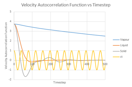
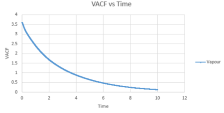
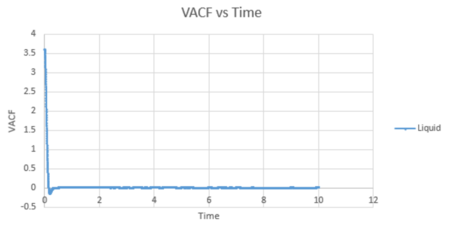
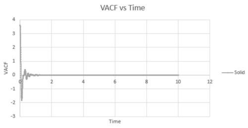
The VACF values calculated from all three states was plotted against timestep, along with the harmonic oscillator VACF for comparison.

Velocity Autocorrelation Function vs timestep

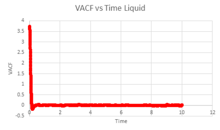
The liquid and solid VACF have a maximum value when the timestep is zero. This can be explained by the fact that at $\tau =0$, $v(t)$ will equal to $v(t+\tau )$ giving a maximum value. The minimum values obtained for the liquid and solid not long after the initial timestep represent the point at which the vectors of velocity are parallel in opposite directions; occurring after a collision as the 'bounce' away from each other. The minimum of the solid is at a lower value than that of the liquid. This may be explained by the fact that the liquid has a larger diffusion coefficient and weaker intermolecular forces, so that once the atoms in the liquid have collided (which are weaker collisions than that for a solid) and bounced away from each other, they diffuse further away reducing the possibility of another collision. In addition, the liquid has only one minimum value, whereas the solid has two, this is due to the collisions of the liquid with the solvent cage, reducing further collisions.

The difference in the atomic motions of solids and liquids explain the main differences between their paths on the graph. The solid system experiences only vibrational motion, whereas the liquid system experiences diffusion within the system. Due to both systems experiencing interatomic forces, they move to be in a position where their atoms are at equilibrium aka where the repulsive and attractive forces balance. This explains the oscillation around zero VAFC observed for the solid; the vibrations of the atom reaching its equilibrium value as it moves backwards and forward, reversing the velocity vector. These oscillations decrease in magnitude as the timestep increases as equilibrium distance is reached. For a liquid, an oscillation is not seen due to the atom positions not being as closely bound compared to that in a solid and consequently their diffusion suppresses any oscillation.

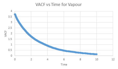
For the vapour, its graph decreases slowly with time and its equilibrium value is not reached within this timestep constraint. This is due to the weak interatomic forces between the vapour atoms as the diffuse apart from each other, reducing their velocity.

The harmonic oscillator graph has a continuous oscillation of the same magnitude. This is because it is assumed in a harmonic oscillator that the atoms are vibrating on a perfect string and therefore do not experience collisions. This results in its velocity remaining constant as there is nothing to disturb its motion.

JC: Good understanding of the VACF. The VACF reaches zero due to random collisions causing atom velocities to become decorrelated.

Vapour VACF vs Time (reduced number of atoms)	Liquid VACF vs Time (reduced number of atoms)	Solid VACF vs Time (reduced number of atoms)

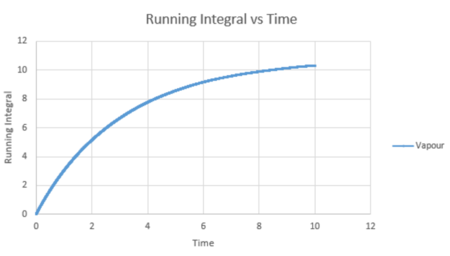
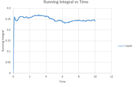
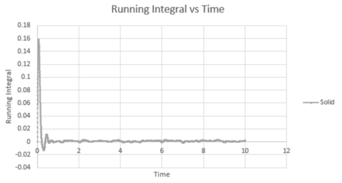
The trapezium rule is a way of determining the area under a curve. We will use this to approximate the integral under the velocity autocorrelation function for each state. These can then be used to calculate the diffusion coefficient. Below shows a plot of the running integral calculated using the trapezium rule.

Vapour VACF vs Time running integral (reduced number of atoms)	Liquid VACF vs Time running integral (reduced number of atoms)	Solid VACF vs Time running integral (reduced number of atoms)

Vapour VACF vs Time (for a million atoms)	Liquid VACF vs Time (for a million atoms)	Solid VACF vs Time (for a million atoms)

Vapour running integral vs Time (for a million atoms)	Liquid running integral vs Time (for a million atoms)	Solid running integral vs Time (for a million atoms)

The diffusion coefficient calculated for each state by dividing the last number in the running integral by three. This seen in the table below.

	Diffusion coefficient for the system with reduced number of atoms (cm2s-1)	Diffusion coefficient for the million atom system (cm2s-1)
Vapour system	3.443	3.269
Liquid system	0.0803	0.09
Solid system	5.59*10-4	4.55*10-5

As was seen using the mean square displacement, the diffusion coefficient was largest for the vapour system and smallest for the solid. The reason for these trends have already been previously explained.

It can be concluded that both methods, MSD and VACF, produce similar values for the diffusion coefficient. However, the VACF method only works if the VACF can be integrated to the time limit of infinity; this is not possible to do practically. As the time to complete the VACF increases, the more noisey the correlation function will be because of the greater number of trapezoids required (which will always have an area slightly less or more that than the actual area under the curve). Therefore, accumulation of this 'noise' when integrating the VACF may result in errors in estimates.